
I would like to continue studying numerical methods because I believe that having a very strong understanding of the topic will make learning future subjects (like physics) easier. I mean, it’s all math at the end of the day.
The goal for this week is to understand the ‘most used’ method - Runge Kutta of order 4 (RK4). As such, we will learn about a couple new methods, in order to really get a feel for why certain methods estimate solutions better than others (without diving too much into the math). Finally, we will code each one in C and run some tests to see how each performs.
The midpoint method, or Runge Kutta order 2 (RK2)
Recall that for the following examples, we are interested in Cauchys problems, where we use a differential equation with an initial condition:
where t0, T, and y0 are given.
The midpont method, or RK2, is a good example to understand how we can derive a more precise method (compared to Euler’s method) with just a little more complexity. We’ll see why this is the case in a future lesson (spoiler: it’s due to higher order error terms, and thus smaller Taylor Series truncation errors).
The equation for this method is:
where, k2 is:
k2 is the slope at … hence the name “midpoint” method. If we compare Euler’s method and this method, it seems that Euler’s method uses the slope at _t0* while the midpoint method uses the slope at .
However, a question arises:
How do we find the slope at time ?
The steps are as follows:
- Find the slope k1 with the Euler method at t0.
- Use k1 to estimate the solution to the function .
- Find the new slope k2 with the Euler method at .
- Go back to the beginning (where t = t0), and use k2 with Euler’s method to estimate the function y(t0 + h).
I suggest that you look at this part of this link because it has helpful graphics as well as derivations to better see these steps in action. This link also has more in depth calculations.
Runge Kutta 4th Order (RK4)
This method considered as - and I quote the author of the book Numerical Recipes in C:
Runge-Kutta is what you use when: (i) you don’t know any better, or (ii) you have an intransigent problem where Bulirsch-Stoer is failing, or (iii) you have a trivial problem where computational efficiency is of no concern. Runge-Kutta succeeds virtually always.
As we will see, the following equation is quite wordy… but with a little intuition it’s quite easy to understand it. This time, we take four slope estimations at each time step to better estimate the approximation of the trajectory of the curve. This method is the most accurate among the methods we have discussed in this series so far.
The equation is the following:
where are slopes calculated at different points. They are calculated as follows:
Again, please take a look at this link on RK4 in order to gain a better understanding ..but if you understood the midpoint method, I imagine these equations didn’t seem so foreign.
C Implementation and a comparison between methods:
I wrote a C program that can help us see the behavior and the result for each method. I chose the differential equation and our initial condition:
which corresponds to the analytique solution: et
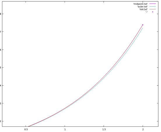
The program writes data to files that we can use with gnuplot with the command plot 'midpoint.txt' w l, 'euler.txt' w l, 'rk4.txt' w l.
Using a small time step h (here I chose 0.025), the three methods are almost equal:
| Method | h | tf | yf |
|---|---|---|---|
| Euler | 0.025 | 2.0 | 7.210 |
| Midpoint | 0.025 | 2.0 | 7.388 |
| RK4 | 0.025 | 2.0 | 7.389 |
| Analytic (et) | 2.0 | 7.389 |
What’s interesting is when we reduce the step size from 0.025 to 1.0, we get the following estimations:
| Method | h | tf | yf |
|---|---|---|---|
| Euler | 1.0 | 2.0 | 4.0 |
| Midpoint | 1.0 | 2.0 | 6.25 |
| RK4 | 1.0 | 2.0 | 7.34 |
| Analytic (et) | 2.0 | 7.389 |
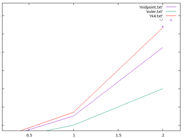
Comparing the three methods we’ve talked about so far, it’s clear that even though the RK4 method takes four times as many steps to estimate a solution at each timestep Δt or h, it can take much larger timesteps to get close to the real value, which may make it way more efficient when compared to other lower order methods!
Next time
I was thinking that I would talk about errors (Taylor series truncation error, global error, local error, etc). However, for the sake of moving on, I think there are plenty of resources online that do a good job explaining them. In any case, if I find a reason explain it in a future subject, I will!
Let’s go to particle dynamics!