Let's Create a Particle System - Part 2

We're creating a particle system from scratch in JavaScript using HTML Canvas and springs.

Keywords: Newtonian forces, numerical methods, maths, physical simulations

By Carmen Cincotti

March 28, 2022

Springs
- Hooke’s law
- The force between two particles
The JavaScript code
The result
Next time
Resources

Last week, I promised you that I would continue my work on particle systems by implementing the example found in Particle System Dynamics under “User Interaction”.

As a reminder, this resource asks us to make a system of particles to simulate a mass-spring system. Last week I developed the basis of the project with a solver that can solve the position of a particle by:

summing up the external forces acting on each one,
finding the acceleration caused by these forces with $a = \frac{\sum F}{m}$
using Euler’s method to solve the velocity and finally the position of the particle.

At the end of this work, our system could only simulate the effect of the force of gravity. This week I’ll be introducing springs: using Hooke’s law, we’ll be able to calculate the forces between two particles when we place a spring between them. I’ll also finish this prototype with a dull, but still lovely UI that will allow us to interact with and configure a simulation in real time.

Springs

Springs will be the star of our project this week. Before seeing the code, let us first take a look at Hooke’s law and how to use this law to calculate the force between two particles.

Hooke’s law

Hooke’s law is defined by Wikipedia:

Hooke’s law is a law of physics that states that the force (F) needed to extend or compress a spring by some distance (x) scales linearly with respect to that distance—that is, Fs = kx, where k is a constant factor characteristic of the spring (i.e., its stiffness), and x is small compared to the total possible deformation of the spring.

where the equation is written as:

F_r = -k_s \Delta l

where F_r is the restoring force of the spring, k_s is the spring coefficient and Δl is the difference in length of the spring between its length when a force is acting on it (which elongates/compresses it), which we’ll represent here has l_f and its resting length r:

\Delta l = l_f - r

Let’s check out a quick example to check our comprehension. Imagine pulling a spring by an arbitrary length Δl:

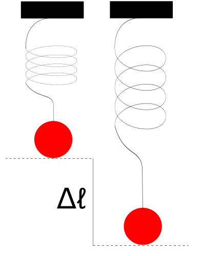
A spring with arbitrary deformation

The spring is pulled by the force of the weight of the ball. The change in length Δl can be measured. For example, if we measure Δl equal to $1m$ and k_s equal to 0.5 $\frac{N}{m}$ , we would calculate the restoring force of the spring using Hooke’s law as follows:

F_r = -(0.5 \frac{N}{m}) * 1m\\ F_r = -0.5N\\

where F_r is negative because the restoring force of the spring wants to act against the force of the ball weight, and is therefore in the opposite direction to the deformation of the spring. That’s because a force isn’t just a scalar - it’s a vector, and vectors have direction too. The restoring force of the spring acts in the opposite direction of the applied forces that cause the spring to deform in order to bring it back to the length of the spring at rest!

The force between two particles

Fortunately, in the resource I often cite, it gives us an equation that we use to solve for the spring force between two particles. We write it:

F_a = \left[k_s(|l| - r) + k_d \frac{\dot l \cdot l}{|l|} \right]\frac{l}{|l|}, F_b = -F_a

Let’s take a closer look at this equation. F_a is like the restoring force, but between two particles it is the force that pulls the particle towards the other until the distance between the two is equal to the length of the spring at rest, r. This is why $F_b = -F_a$ because the force that pulls particle A towards particle B is equal to the negative force that pulls particle B towards particle A, and both approach each other at the same time!

As I said, the length of the spring at rest is the variable r. We can see our first equation:

F_r = -k_s \Delta l

where $\Delta l = |l| -r$ where $|l|$ is the magnitude of the vector distance, l, between two particles. This distance between two particles is a vector which can be found by subtracting the position of one particle from the other: $l = d_b - d_a$ .

Next,

F_d = k_d \frac{\dot l \cdot l}{|l|}

is the damping force of the spring. This damped force is proportional to the velocity of the deformation of the spring. Without it, the system would oscillate forever because the restoring force of the spring is a conservative force, compared to the damping force which is non-conservative. In other words, our system will lose energy over time due to the damping force and therefore will be able to come closer to rest.

Moreover, $\dot l$ is the derivative of $l$ , which is therefore equal to the difference between the velocity of each particule $\dot l = v_a - v_b$

However, the expression $\left[k_s(|l| - r) + k_d \frac{\dot l \cdot l}{|l|} \right]$ will only solve the magnitude of the force, so it will give to us just a scalar value. The direction of the force must therefore also be included in the calculation. To do this, we multiply this scalar by the direction: $\frac{l}{|l|}$ , which is the normalized direction of the force.

At each turn of the loop controlled by requestAnimationFrame, these calculations will be solved by our solver (Euler’s method). Let’s see how I coded it!

The JavaScript code

The code can be found here

I changed a lot of code during this week compared to last week’s code. I’ll let you explore all of that in your free time. I’ll concern myself with reviewing the code pertaining to simulating the physics involved.

Recall that the whole process of calculating the next position of each particle can be summarized as follows:

    loop {
        for particle in the system {
            - advance forward by a time step (deltaTs)
            - add the forces acting on each particle
            - calculate the acceleration of the summed force (F/m)
            - use a numerical method (a solver) to solve the next position of a particle
            - update the Canvas (redraw it)
        }
    }

After initializing our system in the index.html file, we start simulating our system. Here is our new version of the run function:

// Calculate new positions, then draw frame
const run = currentElapsedTs => {
  clearCanvas(ctx)

  // Store deltaTs, as that acts as our step time
  deltaTs = (currentElapsedTs - lastElapsedTs) / 100
  lastElapsedTs = currentElapsedTs

  // Solve the system, then draw it.
  particleSystem.solve(deltaTs)
  particleSystem.draw(ctx)

  if (drawCb) {
    drawCb()
  }
  // Loop back
  requestAnimationFrame(run)
}
requestAnimationFrame(run)

As before, we call requestAnimationFrame to notify the browser that we’d like to run an animation (again, see last week’s post for a more complete explanation).

Next, we come to the most important class method, solve, which is responsible for updating the positions of every particle in the system:

 /**
   * Solve the particle system, which updates all the particles's position
   * @param {number} deltaTs
   */
  solve(deltaTs) {
    ...
    this.forces.forEach((f) => {
      f.applyTo(this);
    });

    this.particles.forEach((p) => {
      EulerStep(p, deltaTs);
    });
    ...
  }

This time we introduce a new force that we have to solve for, which I call in the code SpringForce.

/**
 * A spring force between two particles
 */
class SpringForce extends Force {
  constructor(spring) {
    super()
    this.spring = spring
  }

  applyTo(_pSystem) {
    const { p1, p2, ks, kd, r } = this.spring
    const calculateForce = () => {
      // Vector pointing from particle 2 to particle 1
      const l = p1.position.clone().sub(p2.position)

      // distance between particles
      const distance = l.magnitude()

      // Find the time derivative of l (or p1.velocity - p2.velocity)
      const l_prime = p1.velocity.clone().sub(p2.velocity)

      // Calculate spring force magnitude ks * (|l| - r)
      // The spring force magnitude is proportional to the actual length and resting length
      const springForceMagnitude = ks * (distance - r)

      // Calculate damping force magnitude kd * ((l_prime * l) / l_magnitude)
      const l_dot = l_prime.dot(l)
      const dampingForceMagnitude = kd * (l_dot / distance)

      // Calculate final force vector
      // fa = − [springForceMag + dampingForceMag] * (l / |l|)
      const direction = l.clone().normalize()
      return direction.multiplyScalar(
        -1 * (springForceMagnitude + dampingForceMagnitude)
      )
    }
    const f1 = calculateForce()
    p1.applyForce(f1)

    const f2 = f1.clone().multiplyScalar(-1)
    p2.applyForce(f2)
  }
}

In the SpringForce.applyForce method, we calculate the spring force between two particles. You can see that this is exactly an implementation of our equation above:

F_a = \left[k_s(|l| - r) + k_d \frac{\dot l \cdot l}{|l|} \right]\frac{l}{|l|}, F_b = -F_a

This calculated force will be added to the force accumulator on each particle, which will influence the calculation of its position by the solver!

Finally, we pass the force accumulator to the EulerStep function in order to calculate the position of each particle in the system.

/**
 * Given a particle and a time step, this function updates the given particles
 * position and velocity properties determined by taking a EulerStep
 *
 * @param {Particle} p
 * @param {number} deltaTs
 */
function EulerStep(p, deltaTs) {
  // Calculate acceleration step
  const accelerationStep = p.f
    .clone()
    .divideScalar(p.mass)
    .multiplyScalar(deltaTs) // aΔt = F / m

  p.velocity.add(accelerationStep) // vn = vo +  a*Δt
  p.velocity.multiplyScalar(p.damping)

  // Calculate velocity step
  const velocityStep = p.velocity.clone().multiplyScalar(deltaTs) // vn*Δt
  p.position.add(velocityStep) // xn = x0 + vn*Δt
}

The result

Code result

Working demo of the project

I’ve also added handlers for creating particles, creating the springs between particles, and the ability to change the properties of our springs in index.html. Take a look!

Next time

We keep reading Pixar Physics Simulation Animation Course. I believe that I’ll be reading the part about implicit methods.

Carmen's Graphics Blog