While reading the article on position-based dynamics, I realized that there are quite a bit of mathematical concepts that I don’t understand too well. 😕

For example, in the context of constraints, there are concepts such as the gradient of a function. Moreover, when we talk about the optimization of a function that is constrained, we often talk about the Lagrange multiplier and also the Lagrangian.

In this article, my goal is to demystify these concepts.

The gradient

Before discovering the why of the gradient, I suggest that we first look at how to solve the gradient of a multivariable function such as $f(x,y,z)$. The gradient is a vector consisting of the partial derivatives of the defined function, $f$ :

where $\nabla$ is called nabla. It is sometimes called “del”. It denotes the vector differential operator.

Let’s take an example. I have a function defined as $f(x,y) = 5x + 3xy$. First, we need to find the partial derivatives with respect to the variables $x$ and $y$ as follows:

This gives us a gradient:

That was quite easy to solve! Nevertheless, the importance of the gradient remains a mystery that we’ll uncover in the next section. 🕵️‍♂️

The meaning of the gradient

Let’s imagine that we are at the foot of a mountain, and we wanted to climb it as quickly as possible. We see that the right track is to climb it in the direction of the arrow:

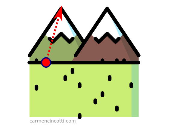
This arrow represents the gradient because it is the fastest ascent up the mountain.

In more precise terms, the gradient vector is the direction and fastest rate of increase of a function $f$ at any given point. This concept is the most important point to remember about the gradient. 💡

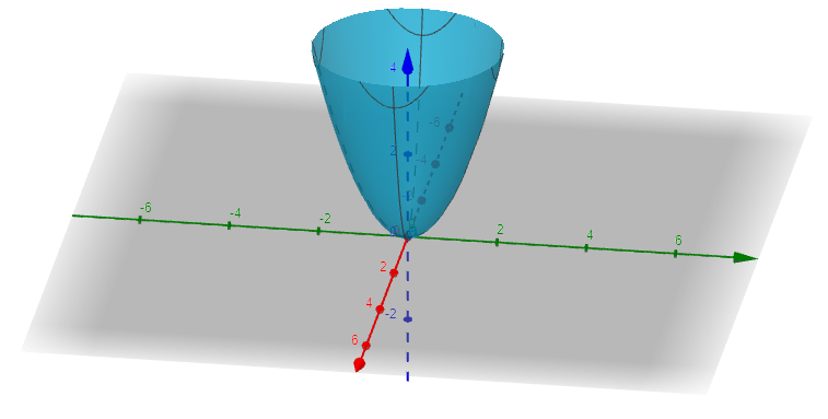
Imagine we create a heat map for a function $f$ within an arbitrary space. Then, we find the gradient at different inputs to $f$ such as $(x_0, y_0, ...), (x_1, y_1, ...), ... ( x_n, y_n, ...)$. If we represent the gradient at each of these points as arrows, we might see the following image:

By Vivekj78 - Own work, CC BY-SA 3.0, Link

We can see that the gradient $\nabla{f}(x, y,...)$ tells us the direction to maximize the value of $f$ at each given input.

Also, the magnitude, $|| \nabla{f}(x_0, y_0,...) ||$, gives us the steepness of this ascent.

Gradient and contour lines

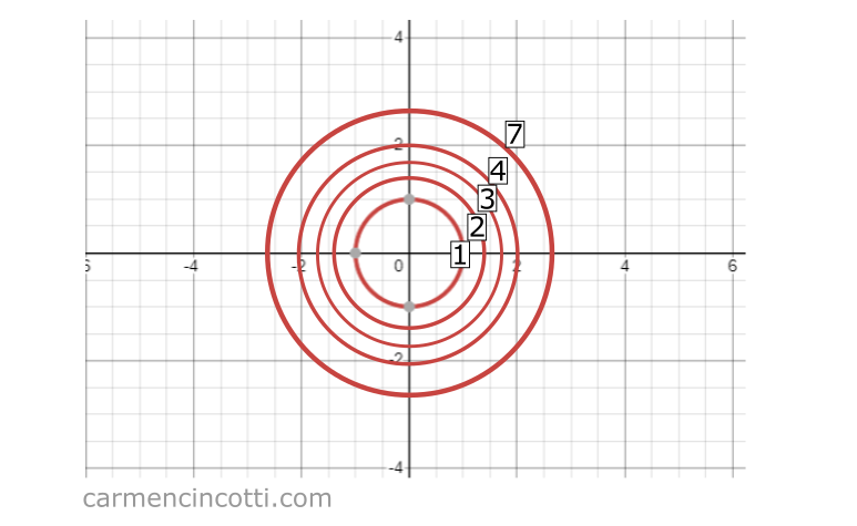
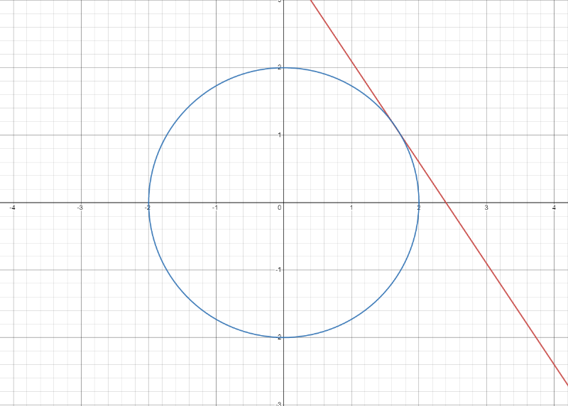
Let’s look at this graph for the equation $f(x,y) = x^2 + y ^2$:

If we squash it from a three-dimensional to a two-dimensional space, we will see these circles which represent the input space, x et y, while the third z value (which represents the output of $f(x,y)$) is denoted by the texts 1, 2, 3, 4, 7:

An important feature of contour plots is that they can help us find the peaks and valleys of a function.

When the lines (at the bottom of the graph above) are far apart, the slope is not steep. Conversely, if the lines are close to each other, the slope is steep.

This is an important point when discussing the relationship between the gradient and a contour plot.

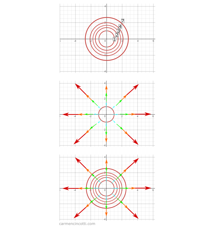
As you can see, each gradient vector is perpendicular to the contour line it touches. This behavior is observed because the shortest track between lines is a line perpendicular to each other.

This makes sense, because we’ve already defined the gradient as the direction and fastest rate of increase of a function $f$.

Application of the gradient - constrained optimization problem

The objective of a constrained optimization problem is to maximize or minimize a multivariable function $f(x,y,z,...)$.

A constrained function takes the form $g(x,y,z,...) = c$.

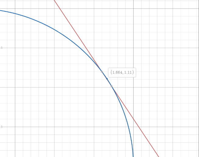
If I take a function $f(x,y)$ and a constrained function $g(x,y)$ such as :

Our goal is to find the point where $f(x,y)$ and $g(x,y)$ are tangential when $c = g(x,y) = 2$:

To do this, we can find the maximum values of $x$ and $y$ using our knowledge of the gradient.

We already know the fact that the gradient points in the direction that is perpendicular to the contour curves.

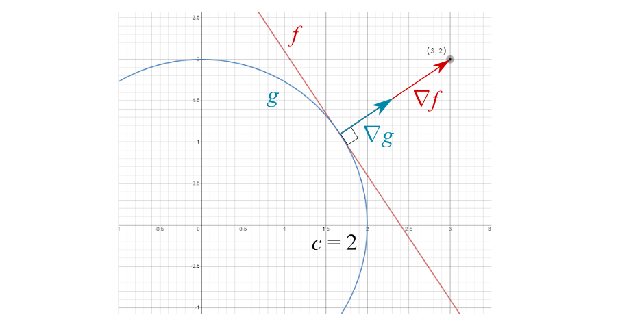
However, the magnitudes of $\nabla f(x,y)$ and $\nabla g(x,y)$ are not the same. We must therefore correct this difference with a scalar, $\lambda$ which is called the Lagrange multiplier:

We already know that to find the values $\nabla f(x,y)$ and $\nabla g(x,y)$, we must take the partial derivative of each with respect to x and y:

We can solve the values $\lambda, x, y$ by solving the following system of equations:

Which gives us the equations:

By solving for $x$ and $y$:

Suppose we want to maximize $f(x,y)$. These points would be tested as inputs to the function. The correct answer would be $(1.66, 1.11)$

The Lagrangian

We can reformulate these functions by writing them in the form:

This function is called the Lagrangian.

Why should I have to write yet another new form of the function? 🤔

In practice, a computer often solves these optimization problems. This shape encapsulates them better. Without a computer, it would probably be easier to separate the functions as we have done before.

For now, I’ll let you do your own research on this subject! Here is a starting point

Resources

• Contour maps - Khan Academy
• The gradient - Khan Academy
• Lagrange multipliers, introduction - Khan Academy
• Lagrange multipliers, examples - Khan Academy