This week was loaded with math! I continued to read Pixar Physics Simulation Animation Course as usual, specifically the article on implicit numerical methods.

This involves solving ODEs (ordinary differential equations) that are considered to be ‘stiff’. We will see why we qualify such ODEs as ‘stiff’ and how we should approach solving for these types of ODEs by using implicit numerical methods such as the Backwards Euler implicit method.

⚠️ Pixar’s resource advises us to avoid an stiff ODE by reformulating our dynamic problem. We’ll be focusing on the cases in which this is not possible.

Stiff EDOs

After having scoured the Internet for a definition of the term ‘stiff ordinary differential equation’, I ended up on Wikipedia’s entry which, admittedly for me, is not very sufficient but I will give it to you anyway:

A stiff differential equation is a differential equation whose sensitivity to parameters will make it difficult to solve by explicit numerical methods.

In short: stiff ODEs are difficult to solve with explicit numerical methods (we talked about explicit methods a few weeks ago).

Definition aside, I find that Pixar Physics Simulation Animation Course gives us a fun example that we will work on to better visualize the Wikipedia definition… Let’s imagine that we want to simulate the dynamics of a particle whose change of position is described by the following differential equation:

where k is a positive and large constant. If k is large enough, the particle will never stray too far from $y(t) = 0$ since $-ky(t)$ will constrain $y(t)$ back to the origin. We also see that the x position of the particle is freer to move around, as described by the absence of this large and positive constant k.

In this example, this ODE would therefore be ‘stiff’ if the variable k is so large that the particle stays close to the line $y = 0$. As we will see in the next part, explicit methods will have a hard time simulating this expected behavior.

The problem with explicit methods

Recall that the equation of the explicit Euler method is described as follows:

and in this example, $X_0 = \begin{pmatrix} x_0 \\ y_0 \end{pmatrix}$ and $\dot X(t) = \frac{d}{dt} \begin{pmatrix} x( t_0) \\ y(t_0) \end{pmatrix} = \begin{pmatrix} -x_0 \\ -ky_0 \end{pmatrix}$. Then, after the substitution, we have:

Which produces the following:

We learned in Part 1 of Numerical Methods that in order to find a solution, we must take small steps in time to approach the solution as massive steps could very well make the system unstable. A quick rearrangement of terms will show us that these conditions must be met in order for the position of the particle described in our example to converge to (0,0):

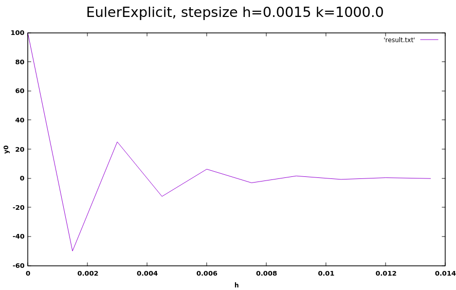
🚨 If we take k equal to 1000: the maximum permitted step is calculated to be $1 - 1000h = -1 => h = 0.002$. If we surpass this limit, the particle’s y position will never be able to converge towards 0!

Solving for y by plugging in parameters h = 0.0015 and k = 1000.0 into a forward Euler solver that I wrote, we can visualize the particle’s y position as it oscillates around zero:

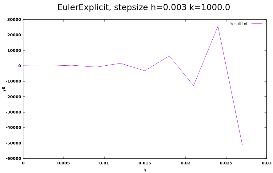
Now, let’s take larger steps in time, where h > 0.002 (h = 0.003 and k = 1000.0). Notice how the solution diverges from 0:

OK, so we could use a very small step like h = 0.0015, right? Maybe… however, we would quickly realize that the x position converges to 0 very slowly, which will make our simulation slow, and expensive!

Can we do better? Could we use a more stable method to converge faster? Yes - with the Backwards Euler implicit method!

Backwards Euler (implicit)

Backwards Euler is the easiest of the implicit methods to understand and that’s why I’m going to focus on it.

Here is the equation:

If you had been an observant person, you would have seen that the difference between the implicit Euler equation and the explicit Euler equation is that the change in X is defined as $h\dot X*{new }$ in the implicit Euler equation. We must therefore solve this change by calculating $\dot X*{new}$… to finally calculate $X\_{new}$.

In fact, it’s like walking backwards.

In other words, it’s as if we were at position $X\_{new}$ and wanted to move backwards to get to position $X_0$… Hence the name: ‘Backwards Euler’.

It’s a little awkward to solve $X*{new}$, since we need to find $\dot X*{new}$… which is also unknown. Let’s see if we can rewrite this into something we can solve.

We start by providing the equation of the Backward Euler method:

where $\Delta X = X\_{new} - X_0$. We can write it as follows:

Using the last equation, we can rewrite our equation for $\Delta X$

We can multiply everything by an identity matrix to isolate our variable $\Delta X$.

After having isolated $\Delta X$, it is now possible to solve $X\_{new} = X_0 + \Delta X$. We will see how to do it with C code in the next part.

Finally, a solution and some code

Here is the code that I will refer to in this section.

As a reminder, we want to converge this stiff ODE:

And we know $\frac{\partial}{\partial X}f(X(t))$ is the Jacobian matrix:

Let’s go back to the equation $\Delta X = (\frac{1}{h}I -f'(X_0))^{-1} f(X_0)$. We calculate $\Delta X$ as follows:

What’s interesting is that you can take a step with any magnitude! If we calculated the limit of $\Delta X$ as it approaches infinity, we would see that:

So $X*{new} = X_0 + -(X_0) = \begin{pmatrix} 0 \\ 0 \end{pmatrix}$ as _h* approaches infinity!

Now we can use the program I wrote to see this example. after navigating to the folder where you downloaded the code, run the following:

where h=0.2, k=1000.0, x₀=100.0 and **y₀ **=100.0. You should see two files implicit.txt and explicit.txt added to the folder. In implicit.txt we see that y converges to zero!

But in explicit.txt it’s a completely different story:

Next time

We will see how to solve stiff second order differential equations! See you next time!

Resources

• Wikipedia - Stiff equation
• Large Steps in Cloth Simulation - CMU
• Implicit vs. Explicit Numerical Methods
• Developing a Matrix Library in C - UNC
• Approximating the Solution to the Cauchy Problem in C++
• Lecture 26 Implicit Euler’s Method - YouTube