Position Based Dynamics | PBD

We're finally ready to start simulating. Through my research, I stumbled across a super performant and exciting way to simulate cloth - through the power of Position Based Dynamics.

Keywords: cloth simulation, numerical methods

By Carmen Cincotti

July 11, 2022Updated September 12, 2022

Advantages and disadvantages
The algorithm
Resources

During the article where we created a Hookean particle system, we used cumulative external and internal forces from which accelerations are calculated based on Newton’s second law to simulate physical effects such as stretching, shearing, and bending.

However, a quasi-new methodology exists that removes the layers of velocity and acceleration, which is called position-based dynamics.

PBD demonstration

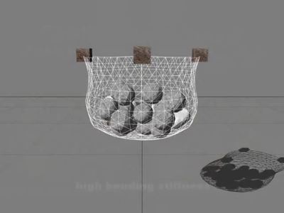
Source : Position Based Dynamics - Matthias Müller-Fischer, YouTube

This method will allow us to solve our system by working directly on the positions of the particles by satisfying constraint functions.

With this methodology, we can simulate fabric as well as fluids, deformations, etc!

Advantages and disadvantages

To begin, I would like to highlight the advantages and disadvantages compared to simulations based on external and internal forces.

Advantages :
- Quick, easy to set up and controllable.
- It avoids “overshooting” problems encountered when using explicit time integration.
- It is able to work with arbitrary constraints as long as the gradient of the constraint function can be determined.
Disadvantages:
- The stiffness of the model depends on the stiffness parameter as well as the magnitude of the time step and the number of iterations of the solver.

The algorithm

for all vertices i 
    initialize xᵢ = xᵢ_₀, vᵢ = vᵢ_₀, wᵢ = 1/mᵢ
while simulating
    for all particles 𝑖 (pre-solve)
        𝐯ᵢ ← 𝐯ᵢ + ∆𝑡*wᵢfₑₓₜ(𝐱ᵢ)
        𝐩ᵢ ← 𝐱ᵢ + ∆𝑡*𝐯ᵢ
    for solverIterationCount
        for all constraints 𝐶 (solve)
            solve(𝐶, ∆𝑡) (solve for 𝐱ᵢ)
    for all particles 𝑖 (post-solve)
        𝐱ᵢ ← 𝐱ᵢ + ∆𝐱ᵢ
        𝐯ᵢ ← (𝐱ᵢ − 𝐩ᵢ)/∆t

Source

Let’s go through this pseudo-code together to better understand it. Suppose we are using a particle that is constrained to a wire, like what you might see on a ‘bead rollercoaster’.

Initialization

Initialization of the particle

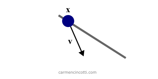
To start the simulation, we need to initialize our attributes. Each particle has three attributes: its mass (m), its position (𝐱) and its speed (𝐯).

Let’s imagine from this scenario that there are two contributing velocities - the velocity of gravity and an initialized velocity in the direction of the wire - which gives a final velocity vector in the direction shown in the image.

After initializing them, we can start updating them in the following steps.

Pre-solve

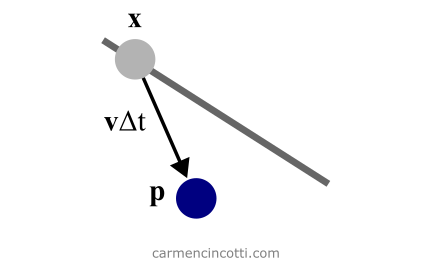
Particle is moved to new unconstrained position

Before imposing the wire constraints, the particle moves in the direction of the velocity vector for a given time interval, Δt.

To do this, we take a Euler step. We have already learned about this numerical method months ago.

Brilliant 🎉! We managed to approximate the new position of the particle! However… it’s no longer attached to the wire! Let’s fix that.

Solve

Move the particle back to the wire

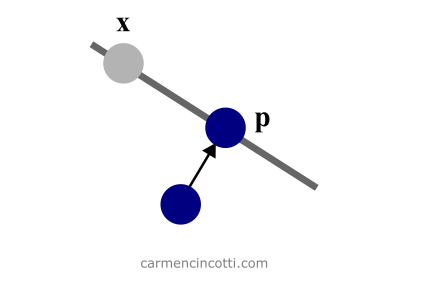
Onward to the beauty of position-based dynamics. The iterative solver manipulates the position of the particle in order to satisfy the constraints.

Constraints

There are two types of constraints:

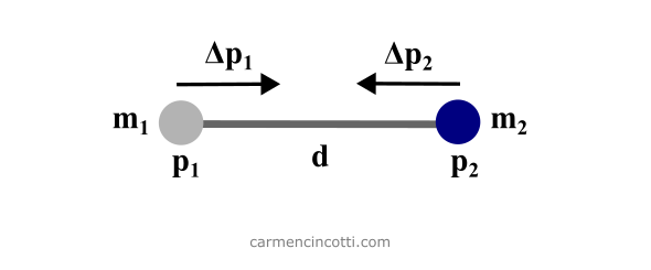
Equality (bilateral) - Equality constraints are constraints that must always be enforced. An example of this type of constraint is a distance constraint where, say, $d = 2$ :

Distance constraint example

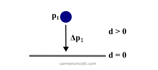
Inequality (unilateral) - An inequality constraint uses the comparison operator $<=$ or $>=$ . There are therefore several solutions that can satisfy such a constraint. For example, here is this particle which is falling to the ground. It will continue to fall as long as $d > 0$ :

Falling ball to ground example

In addition, an important point is that these constraints belong to a group of constraints considered nonlinear. Here is the difference between nonlinear and linear constraints:

Linear - Linear inequality constraints have the form $A·x ≤ b$ . Linear equalities have the form $A·x = b$ .
Nonlinear - Nonlinear inequality constraints have the form $c(x) ≤ 0$ , where $c$ . Similarly, nonlinear equality constraints also have the form $c(x) = 0$ .

The difference between linear and nonlinear systems is beyond the scope of this article, but we may rediscover them soon!

The iterative solver

As I said before, the job of the solver is to move the particle in order to satisfy the constraints.

The problem that needs to be solved comprises of a set of M equations for the 3N unknown position components. However, the number of constraints $M$ is not necessarily equal to $3N$ . In this case, the system is considered as asymmetrical.

Knowing these details, we can consider the system that we have to solve as an asymmetric and nonlinear system with equalities and inequalities. How scary! 👻

The process is iterative as we can see by seeing the loop using solverIterationCount. Also, each constraint is solved individually using a nonlinear Gauss-Seidel solver.

We will see more in a following article. For now, my goal is to present all this knowledge in a high level way.

Post-solve

Post solve step image

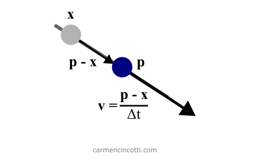
After satisfying the constraints and moving the particle back to the wire, we need to solve for the new velocity. Finally, the loop is repeated!

Carmen's Graphics Blog