
What is Open Addressing?
Open addressing is an alternative method to resolve hash collisions. Unlike separate chaining - there are no linked lists.
Each item is placed in the hash table by searching, (or probing as we’ll call it), for an open bucket to place it.
How is this possible? To better understand this, we must first learn about probing.
What is Probing?
Probing is the method in which to find an open bucket, or an element already stored, in the underlying array of a hash table.
There are a few popular methods to do this. Each method has advantages and disadvantages, as we will see.
- Linear probing: One searches sequentially inside the hash table.
- Quadratic probing: One searches quadratically inside the hash table.
- Double hashing: One searches inside the hash table by hashing a key twice.
How to grow a hash table over time?
To increase the size of a hash table, we take advantage of two tricks to help us - the load factor and a process known as rehashing.
The load factor
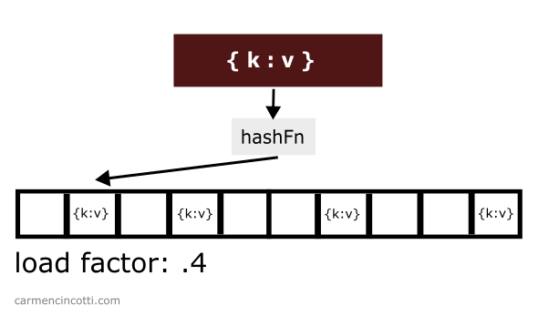
The load factor measures how full a hash table is.
It is defined as where is the number of elements in the table and is the size of the hash table.
Therefore, as we increase the amount of elements in the hash table, the load factor will increase…
This will undoubtedly cause hash table access times to increase over time due to having to deal with hash collision resolution.
But… all is not lost. To help us maintain blazing access speeds, one needs to define a load factor threshold… which when surpassed, will trigger a process within the hash table known as rehashing, which we’ll see now.
Rehashing
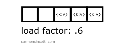
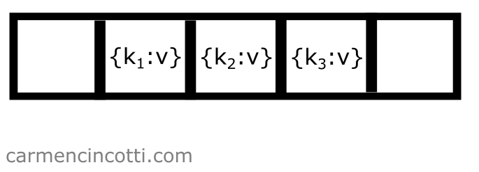
When the load factor threshold is crossed, we must increase the size of the underlying array… generally, we double the size during this process.. Consider this example where I have a hash table with a load factor threshold set to 0.7.
There are already three items stored in the table while the size of the table itself is . The load factor is therefore .
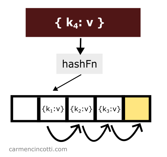
If I add one more element to this table:
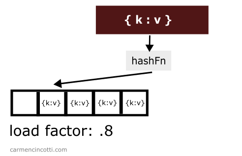
The load factor will cross the threshold! It will then be necessary to double its size in order to reduce the load factor:
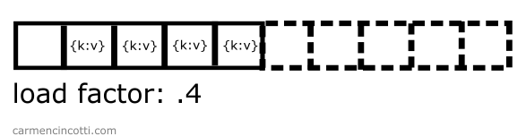
At this point, one must rehash all the elements and put them back in the table.
This process is expensive. This is why we only perform this process when the load factor threshold is crossed.
Time complexity
The time complexity of such a process is . However, this process only happens once in a while.
So for the most part, we’re benefiting from the time complexity that the hash table provides. In this case, the time complexity is said to be amortized at .
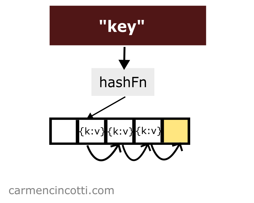
Linear Probing
Linear probing is a way to solve hash collisions by sequentially searching for an open slot until one is found.
The formula is as follows:
where is the index of the underlying array, is the hash function, is the key, and is the iteration of the probe. is the size of the table.
Common operations
The common operations of a hash table that implements linear probing are similar to those of a hash table that implements separate chaining.
We will see what this means in the next sections.
Insertion
Consider the following example - we have an underlying array that is already populated with a few elements:
If we would like to add another element to the table with key which is hashed at the same location of another element, we only need to iterate through the underlying array until we find an open bucket in order to place the element in the table:
Search
Linear probing works as its name suggests. There is a probe that linearly traverses the underlying array. If it finds an element in its path while traversing the array - it will return it to the user.
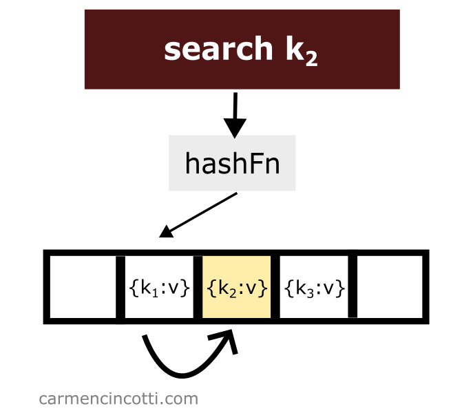
However, if it finds an empty bucket during its search, it will stop at this moment and signal to the user that it has found nothing.
Which raises the question - what will happen if we delete an element? 🤔
Deletion
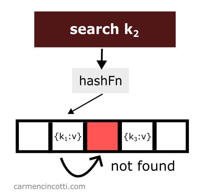
Deleting an item while using linear probing is a bit tricky. Consider this example where I naively remove an item from a hash table:
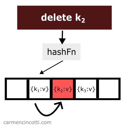
We just deleted an item from the hash table. Then we look for the item which is hashed by the hash function in the same location as the item which was just deleted and which was placed earlier in the hash table to the right relative to the element that has just been deleted:
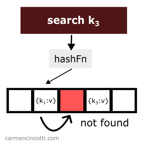
We won’t find it! Why? 🤔
Because the linear probe stops when it encounters a empty space.
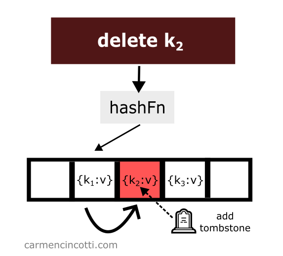
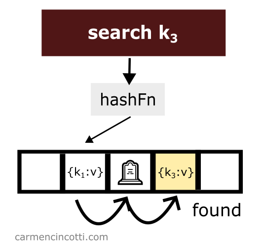
To avoid such unpredicted behavior - we must place at the location of the deletion of an element what is called a tombstone 🪦.
If the linear probe encounters a tombstone while searching the array, it will ignore it, and continue its search for the element we want.
Let’s see an example with this idea in mind:
Then, we search for an element like before, however this time we are able to find it thanks to the tombstone:
Disadvantages
There are a few drawbacks when using linear probing to maintain a hash table. Let’s take a look together!
Clustering
Linear probing is sensitive to a phenomenon called clustering.
Clustering is a phenomenon that occurs as elements are added to a hash table. Elements may have a tendency to clump together, forming clusters, which over time will significantly impact performance for searching and adding elements because we’ll approach a worst case time complexity.
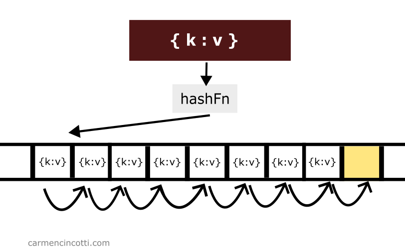
One could say that linear probing is an efficient way to fill a hash table if the table isn’t too full!
Maintenance
During a hash table’s lifetime, one must maintain the underlying array in order to avoid overstocking problems.
As we have already seen, if the array is too full, we risk degrading the time complexity from to .
To avoid this problem, we should keep track of the load factor.
Advantages
There are also a few advantages of using such a structure.
Cache performance
Because linear probing traverses the underlying array in a linear fashion, it benefits from higher cache performance compared to other forms of hash table implementations.
Simplicity
It must be said that the complexity of finding an open space is easy because the probe traverses the underlying array in a linear fashion.
The other methods, as we will see, are sensitive to cycles. This phenomenon occurs when the probe repeats its path trying to find a free space - and this cycle never ends!