
This week I would like to continue the discussion on the graphics rendering pipeline. Last week we touched on the discussion of transforming a vertex from 3D to 2D.
You might be asking yourself:
How do we transform these vertices into pixels?
To answer this, we need to dive into the rasterization process.
Rasterization
Rasterization is the process by which the GPU finds all the pixels inside a primitive (the GPU will only rasterize triangles) using the given primitive’s transformed vertices (each with a z-value and other information associated with this).
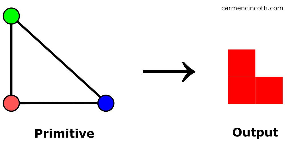
Here’s a GIF that shows us a high-level illustration of rasterization:
Over the duration of the GIF, we see how primitives (triangles) change to pixels. In other words, triangles are rasterized to pixels.
We’ll soon see that this process isn’t so simple if we want a nicely rendered image (because of aliasing), but the rasterization itself is pretty easy to figure out, as we will see.
That being said, our first stop is to learn how the GPU determines if a pixel is within a given triangle, or not.
💡Why does the GPU only work with triangles during rasterization?
Besides being the simplest primitive (after a line and a vertex), there are two important reasons as to why using triangles is advantageous:
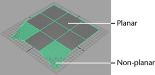
- Complexity - triangles are less complex compared to other higher order primitives. A triangle can never be non-planar.
In other words, all vertices of a triangle exist in the same plane:
- Efficiency - since the triangles are less complex, the algorithms to render them are very fast. Also, triangles require less resources (memory) to render them.
The pixel coverage of a triangle
I’m going to cover this topic in high-level fashion. The hole we can fall into is deep.
That said, I’ll start with our first step: assembling triangles from vertices.
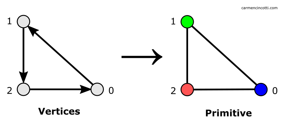
Assembling a triangle (primitive assembly)
The first step in the rasterization process is to stitch together all the vertices that are still visible after the clipping process.
In this step, the edge equations, differential equations, and other information about the triangles are calculated.
Traversing a triangle
Now that we have triangles, the next step for the GPU is to traverse the screen pixels to find the ones inside a given triangle.
With this information, the GPU will determine whether a pixel (or rather, as we’ll see - a sample) is inside a given triangle, or not by running a coverage test.
💡 There are optimizations to avoid traversing all the pixels on a screen. For example, the GPU may limit this traversal to a bounding box that surrounds a given triangle.
First approach - only one sample for each pixel
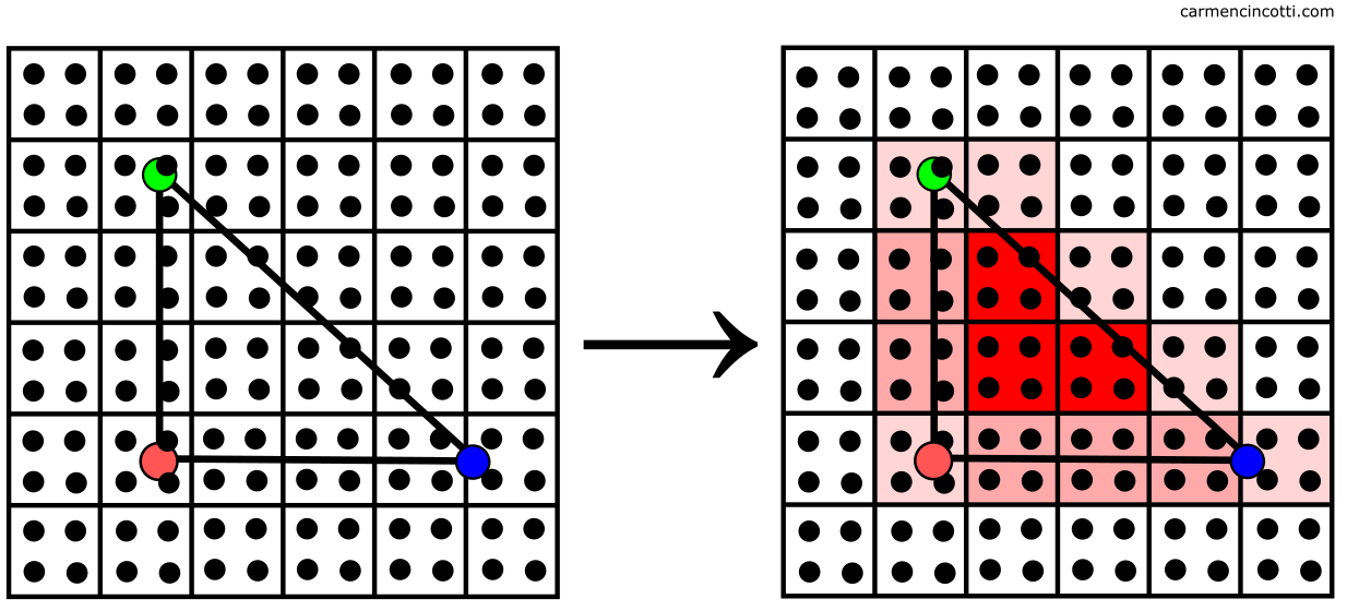
To start, a naive approach is to determine if the center of a pixel is inside a triangle:
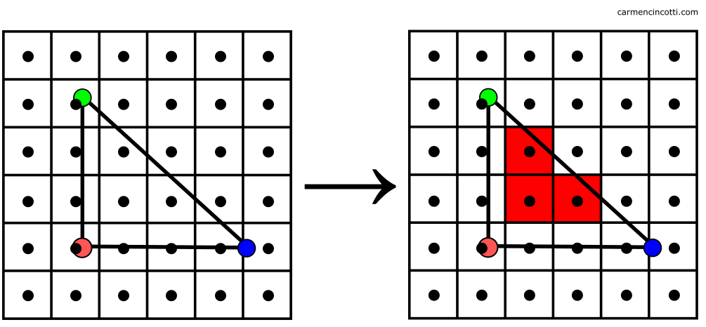
The left grid shows us the output pixels and the dots represent the center of each. On the right, we see the highlighted pixels whose centers are inside the triangle.
But, as you’ve probably already noticed - there will be errors of approximation. Our image will render poorly:
🎉 Congratulations 🎉! We just saw a very well-known problem in the graphics world - aliasing. It is caused by insufficient sampling. Let’s explore these topics a little closer.
Sampling
Sampling is the process of reducing a continuous-time signal to a discrete-time signal. The goal is to digitally represent given continuous information as accurately as possible.
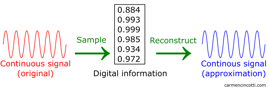
After taking samples, we can take this digital information to approximate the original continuous signal. This approximate signal is called a reconstruction. A filter is used during this reconstruction process in order to re-obtain this approximate continuous signal.
To be clear, our primitives are like continuous signals. We would like to draw them on pixels - a discrete structure.
Therefore, we need to sample our primitives to get the necessary digital information to reconstruct them into colored pixels on our screen. Let’s see this picture again:
As we have already seen: the center of each pixel represents a sample - a discrete location within a pixel. We easily realize that the edges of the output image do not conform to the original triangle.
This problem shows us the constraints imposed by the pixels that we must take into account.
What constraints are imposed?
The constraints are as follows:
- Color - A given pixel can only be one color.
- All or nothing - A pixel is completely colored by this chosen color. It is impossible to color just a small part of a pixel.
Let’s look at a fun example of this rasterized flag :
![]()
Each pixel in the image of the rasterized flag is colored with a single color (red or white) and fully colored with that color.
How many samples should be taken to obtain the best possible image?
The answer is probably best explained in the context of aliasing.
⚠️It must be said that we should only be interested in this idea of what a sample is, and not how they are colored. This will be explained in a future article
Aliasing
Problem 🤔: Recovered signals are never perfectly accurate.
Well, can we at least get close to being perfect?
The sampling rate plays a major role in this case. However, we need to choose a frequency that is both sufficient to accurately recover a given signal without exhausting all of our hardware resources.
That said, undersampling can significantly alter the final recovered signal. Rendering artifacts caused by these undersampling errors are called aliasing.
Here is an animation that shows us how undersampling a signal can effectively render the reconstructed signal useless. The source signal is black, and the recovered signal is in red. The dots on the red line are points where we take our samples :

Let’s rate the sampling rates (ha) that we saw over the course of this GIF :
✅ Start : We see a sufficient sample rate to reconstruct the source signal.
🆗 Middle : The sampling rate is decreasing, but we aren’t losing too much information. We can still be confident that our reconstruction of our source signal is OK.
💥 End : Disaster scenario has been reached. The sampling rate is so low that the recovered signal is completely unrecognizable to its source.
Knowing this, let’s clarify our definition of aliasing:
Aliasing - when high frequencies of an original signal pretend to be low frequencies after being reconstructed due to undersampling.
Let’s see how we can prevent this phenomenon.
Antialiasing - supersampling
If our images suffer from aliasing, we need to increase the sample rate!.
The GPU can sample a pixel multiple times through a process called supersampling. Look at this image where the square is a pixel whose center is represented by a cross:

In this case, we can sample each pixel four times (the blue dots)!
Then an average color value is calculated using the extra pixels for the calculation.
The result is an image with smoother pixel-to-pixel transitions along the edges of the triangles like so:

🎉 Finally 🎉, we’re ready to try rasterizing our image again.
💡*There are several ways to do supersampling*
⚠️It must be said that super-sampling will require more hardware resources and time to render a frame.
Second approach - multiple samples for each pixel
By taking multiple samples and calculating an average color value, the GPU is able to rasterize the primitive as follows:
And finally, we see this much more beautiful image:
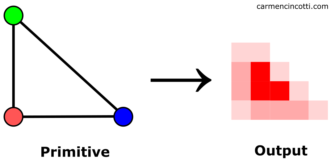
By sampling more times, we’re able to rasterize a primitive that’s much more close to the source primitive than our previous “one-sample-per-pixel” attempt.
Next time
I think the next step is to understand fragments - who they are and how they are processed. See you soon!
Resources
- Computer Graphics (CMU 15-462/662) - Keenan Crane
- Real-Time Rendering, Fourth Edition, by Tomas Akenine-Möller, Eric Haines, Naty Hoffman, Angelo Pesce, Michał Iwanicki, and Sébastien Hillaire
- Rasterization: a Practical Implementation - Scrathapixel
- Supersampling - Wikipedia
- Rasterization and sampling - Imperial College London
- Serious Statistics: The Aliasing Adventure - Overclockers Club
- Intro to Graphics Rendering - Jason L. McKesson
- A Stackoverflow question I found helpful