The PBD Simulation Loop | PBD

Position based dynamics is a fast, stable, and controllable simulation technique that directly manipulates the vertex positions of object meshes in order to model various dynamic and interactive effects of objects such as rigid body, soft body, cloth, or fluids. Let's check out it's simulation loop to better understand how it works.

Keywords: physics, dynamics, linear algebra, multivariable calculus, gradient, linearization

By Carmen Cincotti

August 01, 2022Updated September 12, 2022

The position-based dynamics (PBD) algorithm
The loop
Next time
Resources

We are close to understanding almost everything about position-based dynamics (PBD). While reading these two articles on PBD and its successor XPBD, I quickly realized that there were many concepts completely unknown to me. So, I once again decided to write about them.

I will write this week about the PBD simulation loop, line by line, in order to better understand it all. In the next article, I will write about PBD’s successor, XPBD. At the end, I will choose between PBD and XPBD as a simulation loop to move towards setting up a cloth simulation.

The position-based dynamics (PBD) algorithm

Here is the algorithm to run a simulation with PBD:

PBD Simulation Algorithm

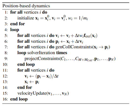
Figure 1 : L’algorithme de simulation de PBD - J. Bender, M. Müller and M. Macklin / A Survey on Position Based Dynamics, 2017

The lines (1)-(3) are to initialize the position and the velocity of the particles because the system is of second order with respect to time: $\mathbf{x_{n+1}} = \mathbf{x_n} + \mathbf{v_n} \Delta t + w \mathbf{f} \Delta t^2$ . Otherwise, there would be too many unknown variables.

Initialization of PBD

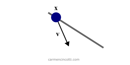
Figure 2 : Initialization of PBD. Particle x is constrained to the line (in gray). It has a velocity of vector v.

Recall that PBD works exclusively and directly on the positions of particles in a system. It is therefore not necessary to maintain the acceleration layer to calculate the velocity and thus the position in the future steps.

The loop

We are now entering the simulation loop! At each iteration, we take a step in time, $\Delta t$ to advance the simulation.

Lines (5)-(6) (of Figure 1) perform a symplectic Euler integration step to advance position and velocity. The new location, $\mathbf{p_i}$ is just a prediction of the final position of the particle not subject to any constraints. We don’t consider constraints until later.

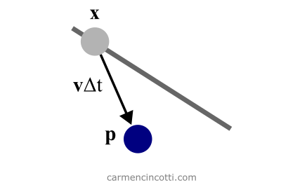
The prediction of the x position of the particle. The prediction is represented by a second temporary variable p

Figure 3: The prediction of the x position of the particle. The prediction is represented by a second temporary variable p.

Symplectic Euler integration

Typical Euler integration advances a system in time $\Delta t$ , or referred to as $h$ here, as follows:

\mathbf{x_{n+1}} = \mathbf{x_n} + h \mathbf{v_n} \\[6pt] \mathbf{v_{n+1}} = \mathbf{v_n} + h \frac{1}{m} \mathbf{f_n}

Note that the velocity $\bf{v}$ is updated after updating the position $\bf{x}$ . However, this method increases the potential energy to the system it simulates. To combat this, we use Symplectic Euler integration:

\mathbf{v_{n+1}} = \mathbf{v_n} + h \frac{1}{m} \mathbf{f_n} \\[6pt] \mathbf{x_{n+1}} = \mathbf{x_n} + h \mathbf{v_{n+1}}

We first determine the velocity of the system in the designated time step, $h$ , then use this new velocity to calculate the position.

In line (7), we continue with the generation of non-permanent external constraints such as collision constraints. We need to generate them at this precise moment to perform continuous collision detection with the new predicted position, $\mathbf{p}$ , from the previous step. I will come back to the subject of collisions in a later article.

The “nonlinear” Gauss—Seidel solver

During rows (8)-(10), a solver iteratively corrects the predicted positions, $\mathbf{p}$ in order to satisfy the constraints defined in the system.

In the article A Survey on Position Based Dynamics, 2017 - Jan Bender , Matthias Müller and Miles Macklin there is this idea of a non-linear Gauss-Seidel solver, because Gauss-Seidel is usually used to solve linear systems. Recall that the difference between the linear constraints and non-linear is:

Linear - Linear inequality constraints have the form $A·x ≤ b$ . Linear equalities have the form $A·x = b$ .
Nonlinear - Nonlinear inequality constraints have the form $c(x) ≤ 0$ , where $c$ . Similarly, nonlinear equality constraints also have the form $c(x) = 0$ .

The Gauss—Seidel method

The Gauss-Seidel method is used to solve a system of linear equations. Recall that a linear equation takes the form:

A\mathbf{x} = \mathbf{b}

Note that this numerical method is iterative. In other words, we use a loop to iteratively approach an approximate solution… which gave me pause. Why do I have to use a numerical method to solve an equation like $A\mathbf{x} = \mathbf {b}$ ? Here is a great resource (slide 2) that answers this question.

Looking at this example of the method in action - we see what is particularly interesting about this method. We substitute the old values for our brand new numerically calculated values during each iteration.

Applying this knowledge regarding the satisfaction of the constraints in the system, we see that each constraint equation will be solved individually and the result of one will immediately get involved in the computation of the other. However, our system has only one constraint to be simpler as an example. Let’s imagine that if there were two that during an iteration, the result of one will influence immediately the result of the others.

In any case, the goal is to solve the constraints like in this image below:

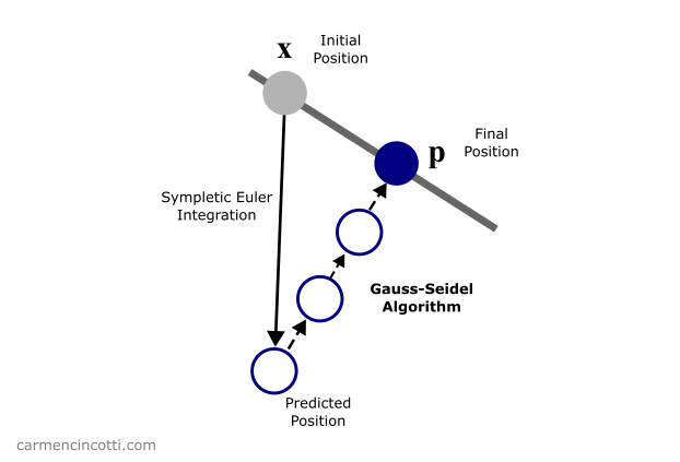
The Gauss—Seidel algorithm in action.

Figure 4: The Gauss—Seidel algorithm in action. The predicted position p is moved to satisfy the constraint (the gray line).

More specifically, we want to iteratively update $\mathbf{p}$ to satisfy our constraints:

Iteration of Gauss-Seidel

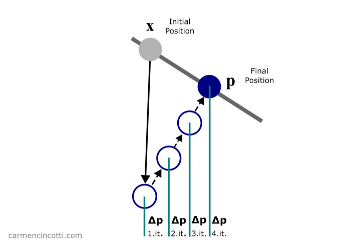
Figure 5: The predicted position p is moved iteratively by $\Delta \mathbf{p}$ to satisfy the constraint (the gray line).

Great! We have a solver ready to help us solve the system 🎉! However, we have a small question that we must answer 🤔:

How do we find $\Delta \mathbf{p}$ ?

Correct the particle position with the Newton—Raphson method

To find the displacement of the particle $\Delta \mathbf{p}$ , we will use a process based on the Newton-Raphson method.

The Newton—Raphson method

The goal of the Newton—Raphson method is to iteratively determine the roots of an arbitrary, nonlinear function. In other words, we minimize this function (assume a function $f(x)$ ) by finding the value of $x$ which will make $f(x) = 0$ .

Let’s take for example this function $f(x) = 0.1x^2 - 1$ . We start by assuming that the value $x = 6$ will minimize the function. We draw a line tangent to the curve $f(x)$ like so:

Graph of equation 0.1 x squared minus one - first attempt

It is clear that $f(x)$ is not minimized by $x = 6$ , because $f(6) = 3.833$ . We continue to search for roots by trying again at $x = 3.833$ :

Graph of equation 0.1 x squared minus one - second attempt

Finally, we repeat this process to finally find the root $(3.1623, 0)$ .

Watch this video to learn more

Following the Newton-Raphson method, we want to linearize the constraint functions. In the case of an equality constraint, it is approximated by linearizing it as follows:

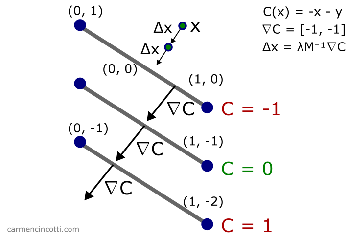
C(\mathbf{x} + \Delta \mathbf{x}) \approx C(\mathbf{x}) + \nabla C(\mathbf{x}) \cdot \Delta \mathbf{x} = 0

To maintain the linear and angular momentum, we restrict $\Delta \mathbf{p}$ to be in the direction of $\nabla C$ :

\Delta \mathbf{p} = \lambda \mathbf{M}^{-1} \nabla C \mathbf{p}^T

where $\mathbf{M}$ is the masses of the particles (we invert them to weight the corrections proportional to the inverse masses). At first sight, I thought to myself uh, what? However, I created some graphs to at least clarify this equation (even if I am still unclear on the conservation of moments).

Imagine that there is a constrained function $C(x) = -x - y$ . The idea is that we want an arbitrary point to stay on this line regardless of external forces:

Constraint chart

We want to minimize $C(x) = 0$ . To do this, we travel in the direction of the gradient of $C(\mathbf{x})$ , $\nabla C(\mathbf {x})$ :

Constraints with gradients

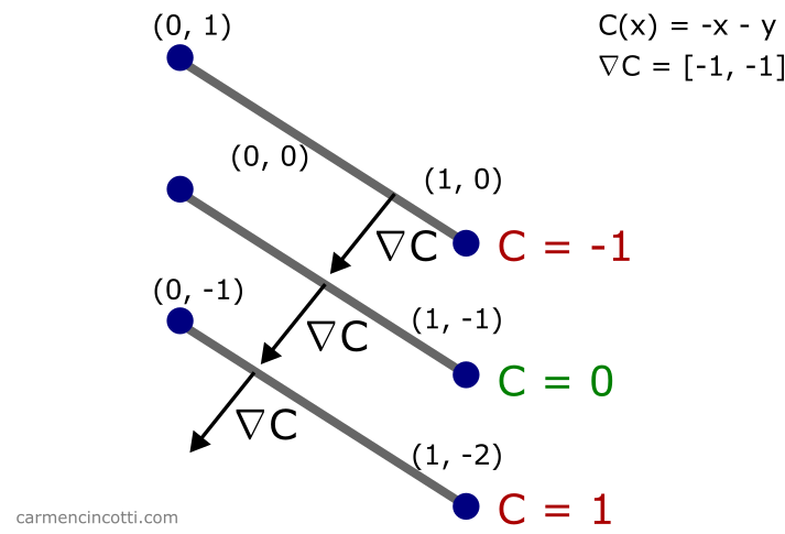
If I arbitrarily place a point $\mathbf{x}$ on this graph and I would like the point to always stay on $C(\mathbf{x})$ - it makes sense that I make it travel in the direction of the gradient of $C(\mathbf{x})$ to get back to line as fast as possible!

Constraints with gradients and example point

Our next step is to find the value of our Lagrange multiplier (a scalar factor) $\lambda$ and then calculate $\Delta \mathbf{x}$ . Rewriting the linear approximation of $C(\mathbf{x})$ is as follows:

- C(\mathbf{x}) = \nabla C(\mathbf{x}) \cdot \Delta \mathbf{x} \\[6pt]

where

\Delta \mathbf{x} = \lambda \mathbf{M}^{-1} \nabla C \mathbf{x}^T

We can perform a substitution to find $\lambda$ :

\lambda = \frac{C(\mathbf{x})}{\nabla C(\mathbf{x})\mathbf{M}^{-1}\nabla C(\mathbf{x})^T} \\[6pt] \lambda = \frac{C(\mathbf{x})}{|\nabla C(\mathbf{x})|^2 \mathbf{M}^{-1}}

After finally finding $\lambda$ and therefore $\Delta \mathbf{p}$ , we update $\mathbf{p}$ .

\mathbf{p_{new}} = \mathbf{p} + \Delta \mathbf{p}

Recall that $\mathbf{p}$ is a temporary positional variable. We update our original position variable $\mathbf{x}$ in the next step.

Then we go through another iteration of the “nonlinear” Gauss-Seidel solver.

The final update of position and velocity with verlet Integration

During the lines (10)-(12) - after the Gauss-Seidel solver, we update the position and the velocity of each particle using an integration method called Verlet integration:

\mathbf{v_i} = \frac{\mathbf{p_i} -\mathbf{x_i}}{\Delta t}\\[6pt] \mathbf{x_i} = \mathbf{p_i}

With Verlet’s integration - instead of storing each particle’s position and velocity, we store its new position $\mathbf{p_i}$ and its previous position $\mathbf{x_i}$ . As you can see, with them we can calculate the new velocity, $\mathbf{v_i}$ !

Then the loop starts again and we start the whole process again! 🎉

Next time

PBD can be extended to provide more visually pleasing simulations by its successor XPBD. We will see that in the next article!

Carmen's Graphics Blog