Cloth Self Collisions | XPBD

Handling self collisions in cloth simulations will make a simulation much more real. This week, we'll study a few tips that Matthias from Ten Minute Physics suggests we use to help us implement this in our own simulations.

Keywords: graphics, tutorial, cloth simulation, leetcode, self collisions

By Carmen Cincotti

November 21, 2022

What is a self collision?
Tips for implementing self collisions
Resources

Self collisions in a cloth simulation are collisions that occur between two particles in a piece of cloth.

Until now, we have been developing a cloth simulation that lives in GitHub.

The handling of self collisions in our simulation makes the difference between a simulation that seems real and one that is not really impressive…

By following this article, we will have a simulation capable of handling self collisions like this:

WebGPU Cloth Self Collisions pic.twitter.com/0uA5lBV2Ce
— Carmen Cincotti (@CarmenCincotti) November 15, 2022

What is a self collision?

A self collision is when two internal particles within an object collide.

Particles colliding

In terms of a piece of fabric, a self-collision occurs when, for example, two threads collide and do not intersect, as in the image below:

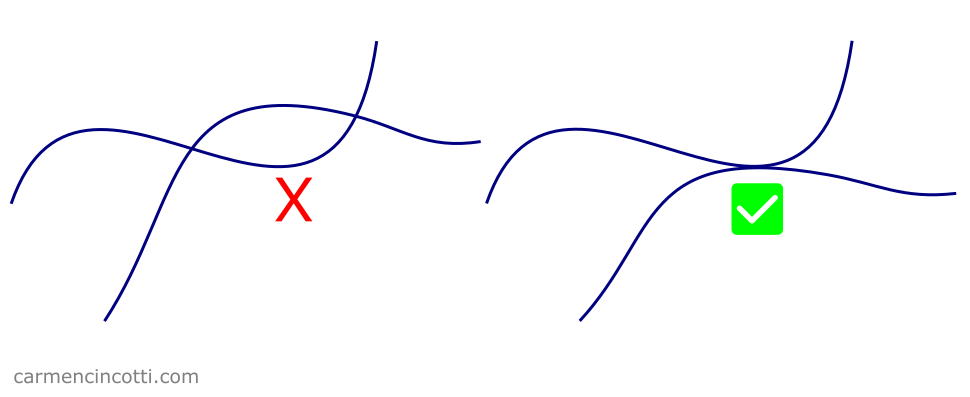
Two threads crossing, which is incorrect. Another showing two threads not crossing, but instead colliding, which is correct behavior.

The two threads on the left cross each other, which is not possible in real life because the threads obey the laws of physics. The two threads on the right exhibit correct behavior because they do not cross.

Tips for implementing self collisions

To implement self collisions into a cloth simulation, I will explain in detail five ideas recommended by Matthias from Ten Minute Physics.

Tip 1: Use a spatial hash table

Fortunately, we have already talked a lot about spatial hash tables!

A hash table

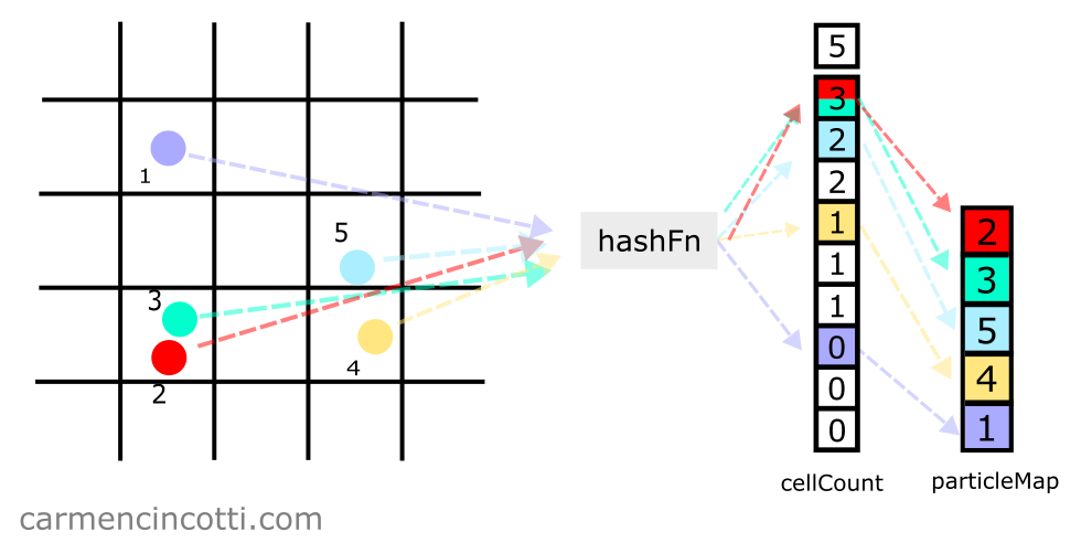
With a spatial hash table, we can detect and correct collisions while looping the XPBD simulation.

We’ll see the code for such an implementation in the next article.

Use uniform particles

That said, to facilitate the use of a spatial hash table, it is recommended to use simple and uniform particles.

Let’s take the following image below as an example:

The uniform particles are located in a spatial hash table (which is represented on the image by the grid)

The uniform particles are located in a spatial hash table (which is represented by the grid in the image).

With this approach, we can simplify all calculations to detect collisions between particles.

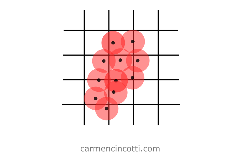
Let’s see the opposite case where the particles are non-uniform:

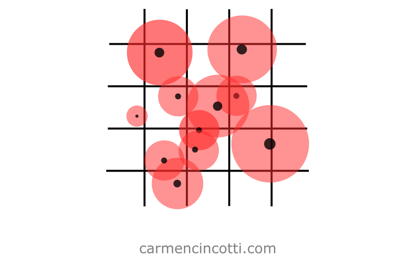
Non-uniform particles in a spatial hash map

By using non-uniform particles, we may have to perform more complex calculations to detect and correct for collisions.

Tip 2: Avoid jerky simulation

In order to have a visually pleasing cloth simulation that takes into account self collisions, we need to consider the values of the following two parameters carefully :

Rest length between particles
Spacing between cells within a spatial hash table

Why consider both?

If these are misconfigured, it may be impossible to reach a stable cloth simulation. Basically, these two settings are linked.

Before seeing why this is the case, let’s review each parameter.

Rest length between particles

Recall that during an XPBD cloth simulation, we define a rest length between the particles:

Distance constraint of a simulation XPBD

In the image above, the variable $d$ is the rest length between each particle in a cloth model.

In XPBD simulation terms, the rest length, $d$ , between two particles acts as a distance constraint, which will constrain the movement of the particles during a simulation in order to satisfy the constraint itself.

Spatial hash table spacing

The spacing is the size of each cell, or “square”, of the imaginary grid which is represented as a spatial hash table in the image below:

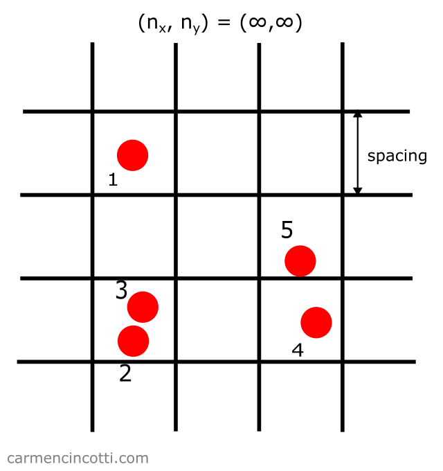
Spatial hash map represented by a grid that has a spacing parameter

This parameter acts as the minimum distance needed between two particles to not be considered a collision, $d_{coll}$ .

The instability problem

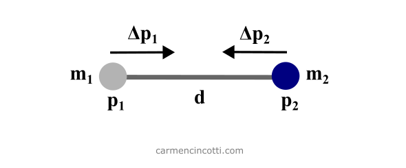
Let’s imagine that I would like to create a simulation with only two particles. I first define the initial position and the radius, $r_p = 0.5$ , of the particles.

Next, I define our two parameters of interest:

The rest length : $d_{rest} = 2.0$
Spacing : Twice the radius of a particle, $d_{coll} = 2r_p = 1.0$ .

Params of an XPBD simulation set correctly

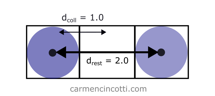
In this case, there is no problem, because the rest length is long enough that $d_{coll} < d_{rest}$ . This means that the distance constraint and the self collision constraint will not fight each other while they attempt to resolve themselves.

However, if I had set $d_{rest} = 0.5$ … it will cause problems:

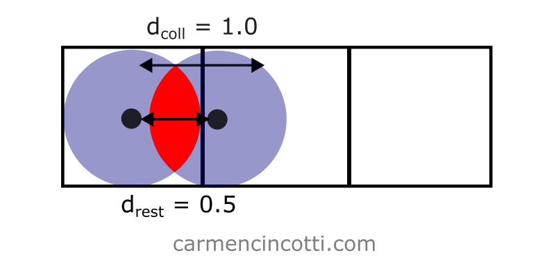
Params of an XPBD simulation not set correctly

In such a simulation, the distance constraint will attempt to resolve itself by bringing the particles together.

However, the self collision constraint will try to resolve itself by acting against this movement.

This will cause a very jerky simulation!

The solution

To avoid a jerky simulation, we must define $d_{coll}$ like so:

d_{coll} = \text{min}(2r_{p}, d_{rest})

By setting $d_{coll}$ like this, the distance constraint and the collision constraint will no longer fight each other in order to resolve themselves.

That said, during a cloth simulation, I suggest defining $d_{coll} = 2r_{p}$ and $d_{rest} > 2r_p$

Tip 3: Use sub-steps

We already learned about implementing substeps to increase the stability of an XPBD simulation a few months ago. We can also use it to better detect and correct collisions between particles:

Collision between two particles, with substeps

Recall that to implement this, we simply need to divide the time step, $\Delta t$ , by the number of desired sub-steps, $n$ .

Next, we will follow the XPBD simulation as follows:

∆𝑡ₛ ← ∆𝑡/𝑛 (substep)
for all vertices i 
    initialize xᵢ = xᵢ_₀, vᵢ = vᵢ_₀, wᵢ = 1/mᵢ
while simulating
    createHash()
    for 𝑛 sub-steps
        for all particles 𝑖 (pre-solve)
            𝐯ᵢ ← 𝐯ᵢ + ∆𝑡ₛ*wᵢfₑₓₜ(𝐱ᵢ)
            𝐩ᵢ ← 𝐱ᵢ
            𝐱ᵢ ← 𝐱ᵢ + ∆𝑡ₛ*𝐯ᵢ
        for solverIterationCount
            for all constraints 𝐶 (solve)
                solve(𝐶, ∆𝑡ₛ) (solve for 𝐱ᵢ)
        for all particles 𝑖 (post-solve)
            𝐯ᵢ ← (𝐱ᵢ − 𝐩ᵢ)/∆tₛ
    render()

This feature in our simulation allows us to avoid a more complex collision detection system like Continuous Collision Detection (CCD). To learn more, take a look at this resource!

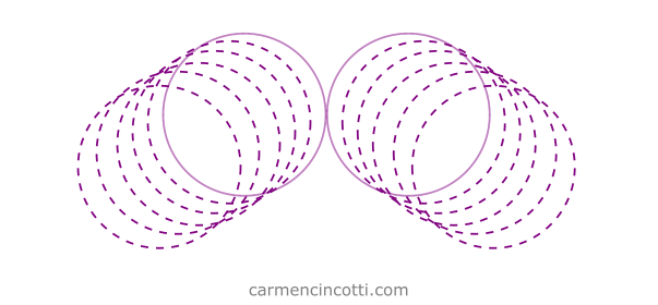
Tip 4: Limit the velocity

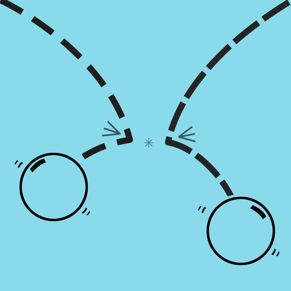
So far, we have a lot of ways to ensure a good simulation. A problem that remains however is the case where the particles in the simulation are moving too fast, which may actualize a phenomenon called tunneling:

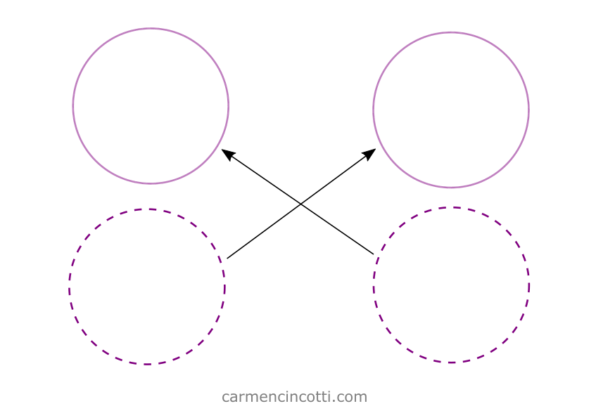
Two particles missing each other curing collision

In the image, we see two particles which were to collide during this time step…

However, they instead went through each other!

A lever we can pull to avoid such behavior is to limit the maximum speed of each particle.

Matthias from Ten Minute Physics recommends that we use this equation to find the maximum permitted speed:

\mathbf{v}_{max} = \frac{r * n_{substeps}}{\Delta t}

where $r$ is the radius of a particle.

We can see with this equation that the more sub-steps, $n$ , that we use, the more the maximum allowed speed increases!

Let’s take an example where I have a piece of cloth containing particles with radii of size $\text{10cm}$ . Our simulation runs with a time step $\Delta t = \frac{1}{60}$ and substeps $n = 20$ :

\mathbf{v}_{max} = \frac{\text{10cm} * 20}{\frac{1}{60}}\\[6px] \mathbf{v}_{max} = 120\frac{\text{m}}{\text{s}}

Using the equation from above, we calculate a maximum permitted velocity of $120\frac{\text{m}}{\text{s}}$ … which is very fast! In a cloth simulation, we’ll probably never come close to surpassing such a high velocity.

Let’s see another example with less substeps and a larger time step: $n = 1$ and $\Delta t = \frac{1}{30}$ :

\mathbf{v}_{max} = \frac{\text{10cm} * 1}{\frac{1}{30}}\\[6px] \mathbf{v}_{max} = 3\frac{\text{m}}{\text{s}}

We calculated a maximum speed of $3\frac{\text{m}}{\text{s}}$ , which is the speed of a human walking!

We can realistically believe that the particles of a cloth simulation could move faster than this.

So, to avoid any potential issues with tunneling, we should cap the velocity of the particles to not surpass this maximum velocity threshold.

Tip 5: Introduce friction

Finally, it is recommended by Matthias to introduce friction during our calculations in order to better stabilize the simulation during a collision.

We should introduce it during the constraint solver loop, more precisely by following the calculation and the positional correction of a particle which has just collided with another particle.

How to calculate the friction correction

Imagine that we have just calculated the new positions $x_1, x_2$ of two particles which have just collided with each other. The next step is to calculate the velocity of each particle by using Verlet integration.

\mathbf{v_1} = (\mathbf{x_1} - \mathbf{p_1}) / h \\[6pt] \mathbf{v_2} = (\mathbf{x_2} - \mathbf{p_2}) / h \\[6pt]

Next, we calculate the average velocity.

\mathbf{v_{avg}} = (\mathbf{v_1} - \mathbf{v_2}) / 2 \\[6pt]

Then we find the difference between $\mathbf{v_{avg}}$ and each already calculated velocity $\mathbf{v_{2}}, \mathbf{v_{1}}$ :

\Delta {\mathbf{v}_1} = \mathbf{v_{avg}} - \mathbf{v_{1}}\\[6pt] \Delta {\mathbf{v}_2} = \mathbf{v_{avg}} - \mathbf{v_{2}}\\[6pt]

Finally, the positions are updated by adding $\Delta \mathbf{v}_i * d$ where $d$ is a damping factor which is between $0$ and $$ $1:

\mathbf{x_1} \leftarrow \mathbf{x_1} + (d * \Delta {\mathbf{v}_1}) * h \\[6pt] \mathbf{x_2} \leftarrow \mathbf{x_2} + (d * \Delta {\mathbf{v}_2}) * h \\[6pt]

I genuinely do not really understand the reasoning behind using average velocity during these steps… so if you know please contact me!

Carmen's Graphics Blog