
A spatial hash table is a special kind of hash table, which is a topic we’ve talked about a lot before in great detail.
Spatial hash maps deal with positions in space.
A spatial hash table is a good tool for detecting collisions between objects and particles, which will prove useful for things such as cloth simulations, video game physics engines, etc.
Let’s see together how such a structure works!
A review of hash tables
Hey! Before continuing on - if you haven’t already read the previous articles on open addressing and hash tables, I really recommend that you take a look so that you can more easily follow along:
What is a spatial hash table?
A spatial hash table looks like an ordinary hash table. However, the most striking difference is that a spatial hash table uses locations (2D or 3D) in space as the keys to hash to enter the table.
Let’s check out an example.
An example
For this example, there is a particle that has settled in space at position .
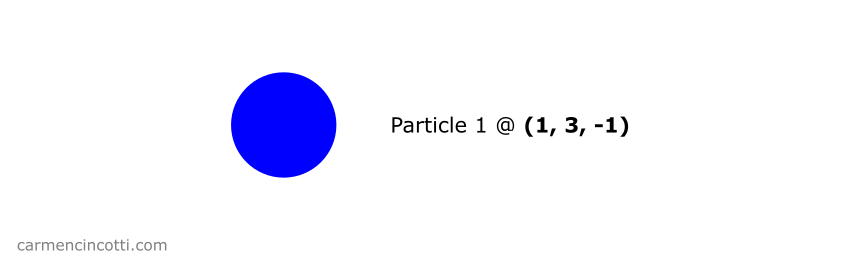
To store this particle in a hash table, we use a hash function which takes as inputs the position of the particle.
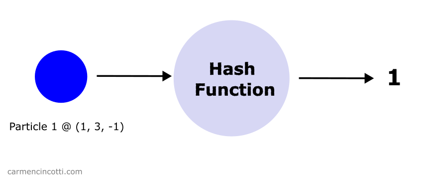
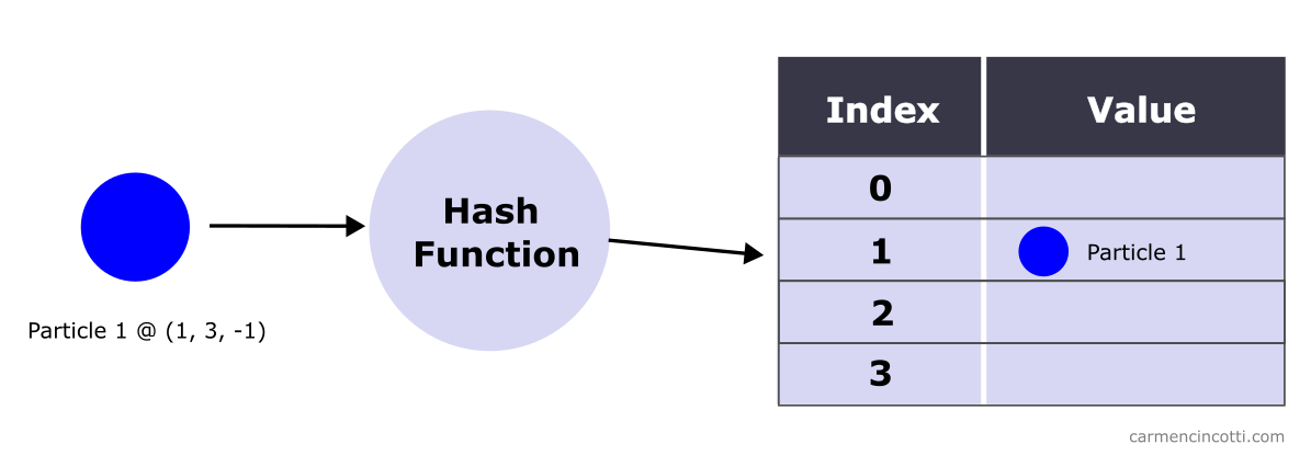
The hash function returns an integer which serves as the index into the spatial hash table. The particle is stored at this index.
How to hash a position
I use this function which comes from Matthias Müller:
  hashCoords(xi: number, yi: number, zi: number) {
    const hash = (xi * 92837111) ^ (yi * 689287499) ^ (zi * 283923481);
    return Math.abs(hash);
  }
The idea is to return a pseudo random integer. Thus, the hash function is less susceptible to returning hashes that cause hash collisions.
Dense spatial hash table
A dense implementation of a spatial hash table was offered by Ten Minute Physics author Matthias Müller during one of his videos.
The dense implementation offers us a very efficient time and spatial complexity.
Only two arrays are used. :
- Particle Array - It stores references to the particles itself.
- Count Array - It stores the number of particles hashed to a particular bucket, which ultimately act as the index into the Particle Array.

We’ll see how this works in the next part!
How to populate a dense hash table
To clarify this idea, let’s see step by step how to populate a dense hash table.
Bounded space
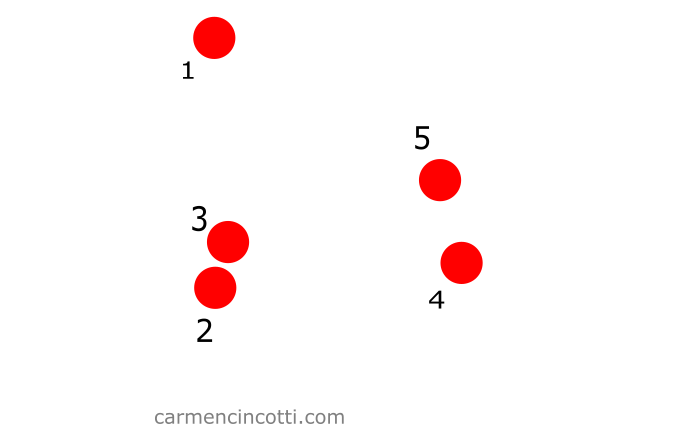
We start with five particles in space like so:
Step 1: Create a grid
Let’s imagine that we create a grid overlaid on our particles:
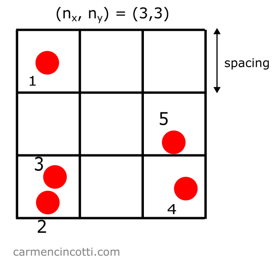
Let’s define some properties of this grid:
- Spacing: the size of each grid square. A good rule of thumb is to define the spacing as two times the radius of a particle, .
- : the number of squares in each direction (and in the 3D case).
At this point, it’s our job to create a table that represents such a grid. Because this array is going to be designated to keep count of the particles in each square of the grid - we’ll call it cellCount:
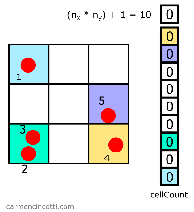
Add an extra space
Note : We add one more space which will be useful when we make a request - or query - for the particles which are around a location of interest. Ignore this for now, we will revisit this later!
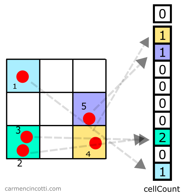
Step 2: Fill the count array
Then, we loop through all the particles to fill cellCount. For each particle that belongs to a particular bucket, we increment the counter by .
How to calculate the bucket that a particle belongs to
We use a particle’s position. Here is a potential method to calculate the index that we will use to index into cellCount :
… and in 3D:
So having a particle at position and a table with size of and with spacing equal to gives us:
The index is equal to .
As you probably have already realized, this example we just saw depends on several variables, like location of the origin. Use this example as a guide and not as a solution.
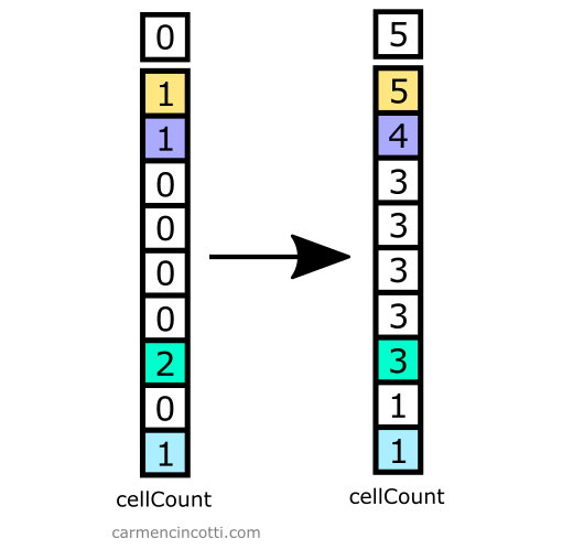
Step 3: Calculate the partial sum
The next step is easy. We need to calculate the partial sum over the cellCount array. We can overwrite it with these new values.
Step 4: Fill in the particle array
Finally, we iterate over all the particles to store them in the array particleMap.
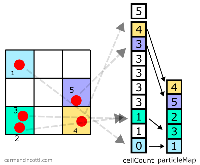
Take for example particle :
- Tout d’abord, on index dans
cellCountà l’indice , car la particule s’y trouve. - Then we decrement
cellCountat this index which thus changes the integer stored here from to . - This new integer is used as the index in
particleMap. We store the particle at index inparticleMap.
You can of course make this method more efficient by combining a few steps to avoid using extra loops.
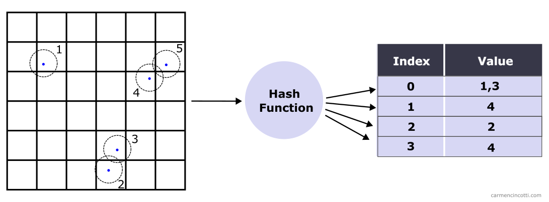
Unbounded space
Let’s start with five particles in unbounded space like this:
Please note that in this example, the space is unbounded. The process from the previous section is therefore no longer sufficient!
Step 1: Create a grid
In this case, the grid is unbounded:
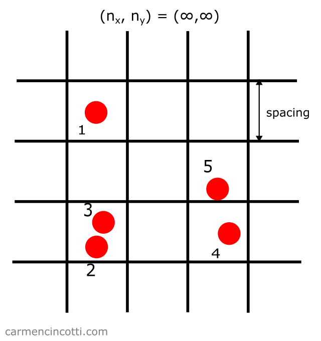
It is therefore not a good idea to try to represent such a structure with an underlying array of storage of an equal size, because we risk wasting too much memory.
How can we avoid this problem?
The answer: We create an array of fixed size to add all the particles to. This implementation will require resolving hash collisions!
Two parameters must be defined:
- Spacing: the size of each grid square. A good rule of thumb is to define the spacing as two times the radius of a particle, .
- Table Size: The size (
tableSize) of the underlying storage table (cellCount).
In this case - we set tableSize to be equal to 9 plus 1 which makes 10:
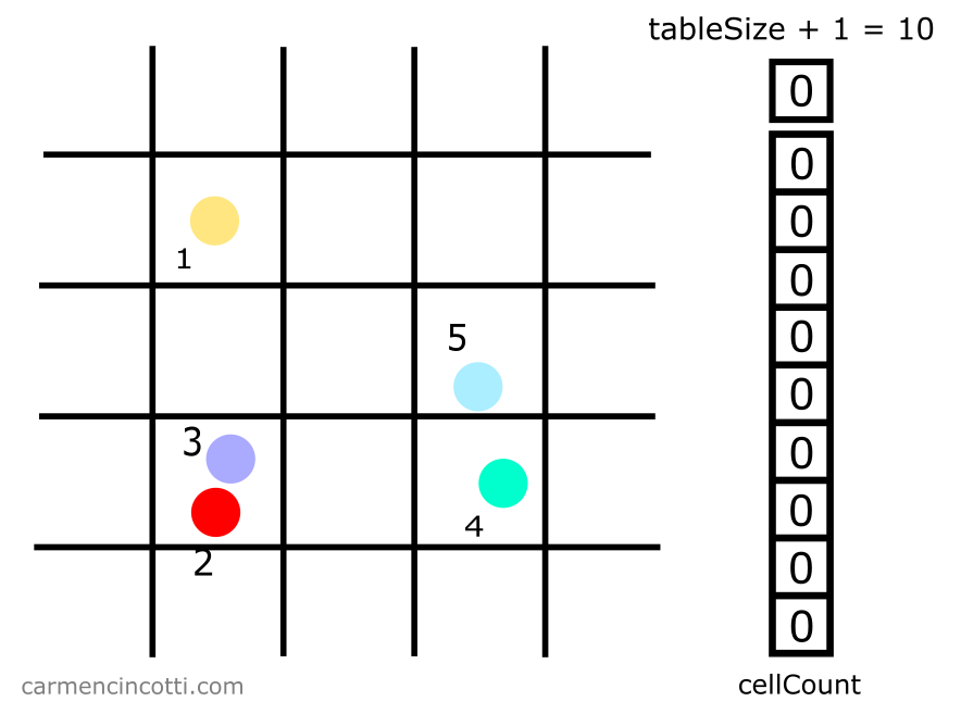
Step 2: Fill the count array
Then we loop through all the particles to fill cellCount. This time we’re using a hash function to index into cellCount. in order to insert particles.
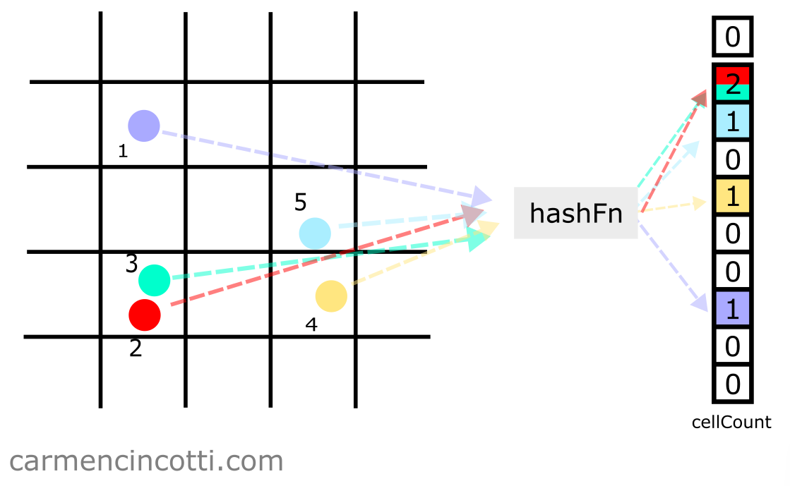
In order to index in the array, we can use this formula:
But what is and ? We could naively define them as the coordinates of the particle itself, but that would mean that particles within the same square could potentially hash to different buckets!
Therefore we have to normalize the coordinates of a particle to instead the position of the square that it resides in.
This is simple - we can use the hashPos function which calls intCoord, which returns a coordinate of a square in the grid :
 intCoord(coord: number) {
    return Math.floor(coord / spacing);
  }

  hashPos() {
    return hashCoords(
      intCoord(pos_x),
      intCoord(pos_y),
      intCoord(pos_z)
    );
  }
And we already defined our hash function, hashCoords, above.
We can now guarantee that all particles within a certain square in the grid will hash to the same location.
How to resolve hash collisions
As you can see, the particles and resolve to the same bucket. We just have to increment the count in cellCount at this index. We will see why it works in the following steps.
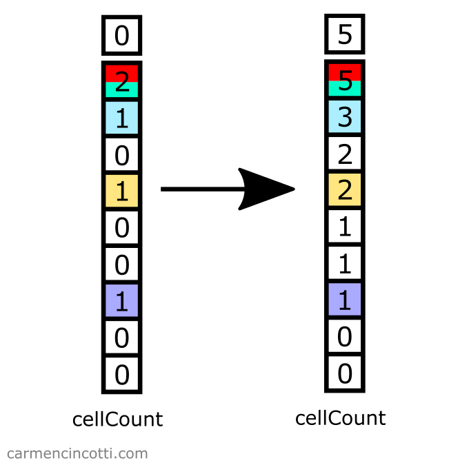
Step 3: Calculate the partial sum
Just like before, we need to calculate the partial sum over the cellCount array. We can overwrite it with these new values.
Step 4: Fill in the particle array
Finally, we iterate over all the particles to store them in the array particleMap (the particle table).
Take for example the particle :
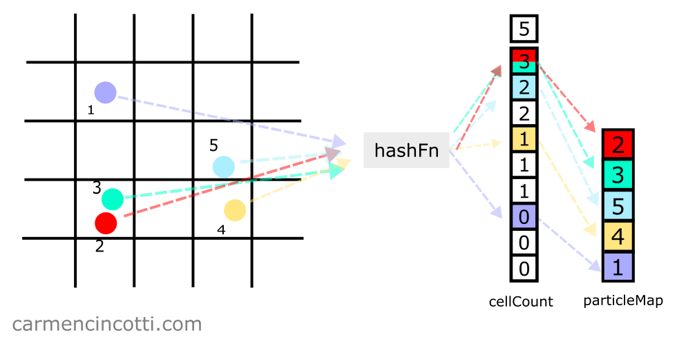
- First, we index into
cellCountat index , because particle is hashed to that location. - Next, we decrement
cellCountat this index, which changes the integer stored here from to . - This new integer is used as an index in
particleMap. Thus, we store the particle at index inparticleMap.
Next time…
We will see how query for particles within the spatial hash table, and of course we’ll start coding!