
A big piece of the XPBD puzzle, which we already talked about a few weeks ago, is the satisfaction of particle constraints. Particle constraints force a particle to move in a certain way, relative to the other particles in the system.
If you’ve been following me for the past few months, you most likely know of my goal to simulate fabric 🧵. Such a simulation may have complex constraints but for now we will only consider distance constraints and bending constraints.
Here are those famous articles that we already studied together during an article a few weeks ago on XPBD that I will reference for the math during this post:
A summary of XPBD
Recall that the XPBD algorithm with small steps is defined as follows:
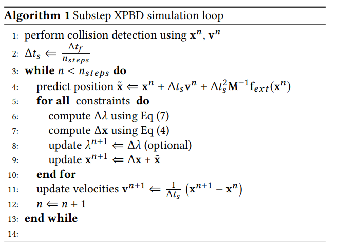
⚠️ As I said, we have already covered this algorithm thoroughly, and I recommend that you read the article if you are already lost.
For now, we are only interested in the loop that is in lines (6) - (11). As you can see, the function of this loop is to satisfy the constraints of the simulation in order to directly correct the positions of each particle that participates in the constraints.
We just covered the reason why this simulation method is called as Position Based Dynamics - PBD 🎉.
Satisfying the constraints
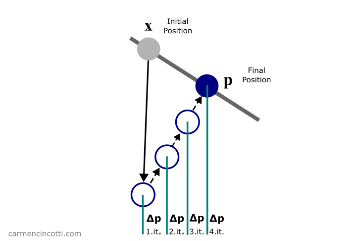
Our objective during the loop is to calculate the correction vector that a particle must move in order to satisfy, or come closer to satisfying, the constraints.
where is defined as:
Note that where is the constraint compliance. Recall that where is the stiffness of the constraint. is the constraint equation, is the gradient of and is therefore a vector. is a diagonal matrix of inverse masses of the particles participating in the constraint.
, , and are scalar values.
Using these equations, we will simulate some constraints with code! 🖥️
The distance constraint
To start, we will talk about the distance constraint because it is rather easy to understand. The objective is to satisfy the constraint by moving two particles so that they approach each other at the rest length, :
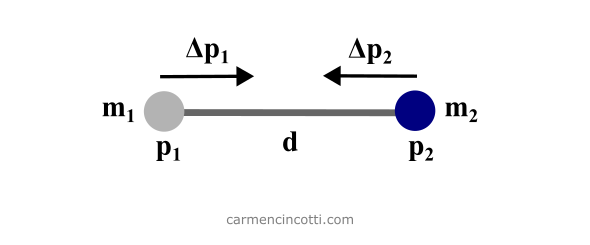
where is the position of a particle and is the mass.
We can solve the equations from the last section in order to find the final position corrections, :
The code solution
Here is the code where I define two particles. The distanceConstraint function is based on calculating and immediately updating the position, of the particle . There is a distance constraint with rest length equal to .
You may notice that there is a little trick during the calculation. Recall that the calculation to find is:
Fortunately, is a normalized vector. So:
We can therefore simplify our equation as follows:
Finally, I used a logging function to see how the particles move before and after the simulation loop:
BEFORE APPLYING XPBD LOOP
-------------------------
POSITION P1:  [ '2.0000', '2.0000', '0.0000' ]
POSITION P2:  [ '-2.0000', '-2.0000', '0.0000' ]

AFTER APPLYING XPBD LOOP
------------------------
POSITION P1:  [ '0.3536', '0.3536', '0.0000' ]
POSITION P2:  [ '-0.3536', '-0.3536', '0.0000' ]
We see that the two particles approach each other and move to the points . Do these new points satisfy the distance constraint? Recall that the length of rest is equal to :
Yes! The distance constraint has been satisfied!
Next time
We will see together the isometric bending constraint. Stay tuned!