
A big piece of the XPBD puzzle, which we already talked about a few weeks ago, is the satisfaction of particle constraints. Particle constraints force a particle to move in a certain way, relative to the other particles in the system.
If you’ve been following me for a few months, you probably know of my goal to simulate cloth 🧵. For the past few weeks, we’ve been talking about the distance constraint and the isometric bending constraint. This week we will be focusing on a more performant bending constraint.
Why change course? Because the isometric bending constraint is expensive to solve 🥵. Matthias Müller shows us an alternative to simulate bending with great results !
Here are once again those famous articles that we already studied together during an article from a few weeks ago on XPBD that I will reference for the math during this post:
A summary of XPBD
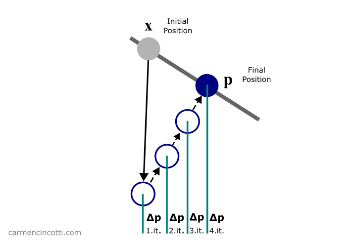
Recall that the XPBD algorithm with small steps is defined as follows:
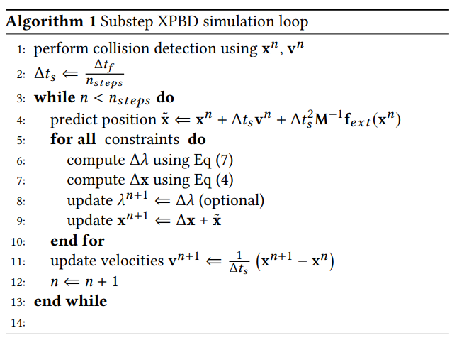
⚠️ As I said, we have already covered this algorithm thoroughly, and I recommend that you read the article if you are already lost.
For now, we are only interested in the loop that is in lines (6) - (11). As you can see, the function of this loop is to satisfy the constraints of the simulation in order to directly correct the positions of each particle that participates in the constraints.
We just covered the reason why this simulation method is called as Position Based Dynamics - PBD 🎉.
Satisfying the constraints
Our objective during the loop is to calculate the correction vector that a particle must move in order to satisfy, or come closer to satisfying, the constraints.
where is defined as:
Note that where is the constraint compliance. Recall that where is the stiffness of the constraint. is the constraint equation, is the gradient of and is therefore a vector. is a diagonal matrix of inverse masses of the particles participating in the constraint.
, , and are scalar values.
Using these equations, we will simulate some constraints with code! 💻
The best performing bending constraint
In this presentation by Matthias Müller, Matthias shows us an alternative to integrate a bending constraint without making complex and expensive calculations. Fortunately, it is very similar to the distance constraint that we already talked about a few weeks ago in this article.
Here is an image that shows exactly what we’re trying to accomplish:
As you can see, there is just one distance constraint between two particles of two adjacent triangles. Of course, this method is a little more complex than a normal distant constraint because you first have to find what triangles are adjacent to each other.
Afterwards, we follow the same process we followed to satisfy the distance constraint. 😮💨
We can solve the equations from the last section in order to find the final position corrections, :
The code
Fortunately, we will see that the code for this constraint is almost similar to the distance constraint. Before seeing it, we must first understand how to find two adjacent triangles.
How to find adjacent triangles
Let’s imagine that we load in a mesh to play with that consists of 1,000 triangles. How could we figure which triangles are adjacent to each other? Fortunately, there is a little trick :
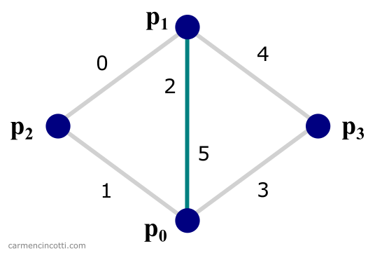
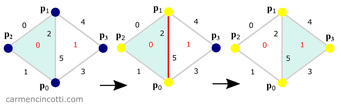
As you can see, there are two triangles that share an edge (2 and 5). We can exploit this fact! Our steps are as follows:
- Create an array where we can search for shared edges between two triangles.
- Use this array to find the four points that form two triangles, as in the picture above.
We first create a list that consists of the edges with ids global that are between each pair of particles. It’s our job to label each edge.
For example, imagine we create a list of edges from this image:
| p_id0 | p_id1 | ei |
|---|---|---|
| 0 | 1 | 2 |
| 1 | 2 | 0 |
| 2 | 0 | 1 |
| 0 | 3 | 3 |
| 3 | 1 | 4 |
| 1 | 0 | 5 |
You can probably see that the particles and share global edges (2) and (5). To find this pair in the code, we sort the edge array in ascending order by the particle id number in each pair:
| p_id0 | p_id1 | ei |
|---|---|---|
| 0 | 1 | 2 |
| 0 | 1 | 5 |
| 0 | 2 | 1 |
| 0 | 3 | 3 |
| 1 | 2 | 0 |
| 1 | 3 | 4 |
Next, we create an array of neighbors, or neighbors in English, which is initialized with -1s, where -1 means ‘no neighbor’. If we create an array of neighbors correctly, we would see an array of neighbors as follows:
Here is the code for a function, findTriNeighbors, which will helps us create this neighbor list:
If you have followed my posts up until now, you will know that I only use WebGPU and JavaScript, without a library like ThreeJS. I say this because you will need to access the index buffer that we have already discussed in this article.
This list of neighbors will be essential for the next step.
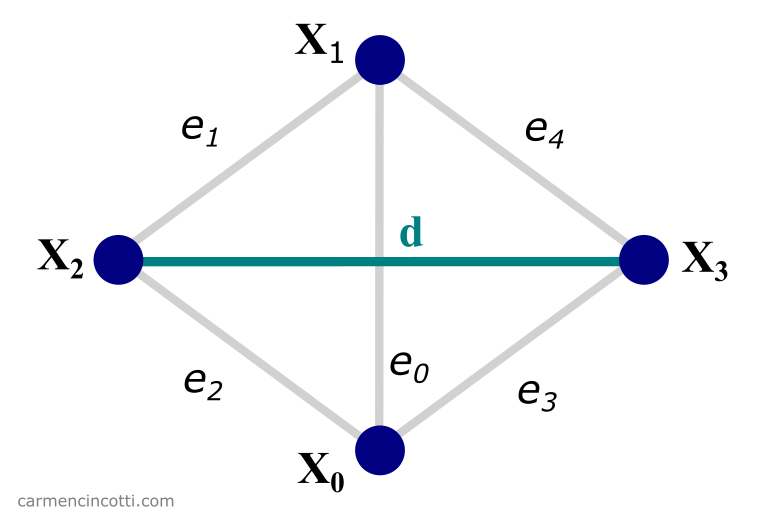
With our neighbor array, we have to create a list containing the identifier of each particle in the quartet that forms each pair of triangles. It will be used to place a distance constraint between opposing particles as in the image below:
The process of doing so is shown in the image below:
We visit each face of our mesh to determine if there is a shared edge (by searching the list of neighboring edges, neighbors). If so, we save the three vertices of this triangle and then we visit the adjacent triangle - where we save the fourth vertex in the configuration.
Here is the getTriPairIds function which does exactly that:
With our list of triPairIds, we are ready to move on to satisfying the constraint! 🎉
The performant bending constraint code
So as you can see, this code is almost the same as the distance constraint code. Just use the two vertices that are not shared instead of just any two adjacent vertices when calculating final position corrections!