
I would like to continue our conversation about spatial hash tables, which we were started learning about last week.
Spatial hash maps will allow us to implement a very important feature of cloth simulations : self collisions.
What is a cloth self-collision?
A self-collision is the interaction that occurs when particles of a piece of fabric collide against one another.
How to query a spatial hash table
Let’s see together how to make queries to a spatial hash table in order to detect particles close to each other, while keeping time complexity fast.
Step 1: Create the spatial hash table and populate it
We have already seen how to do this in the previous article. I suggest you read it before continuing!
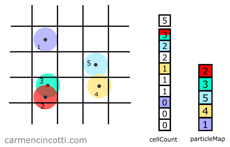
With our two arrays, cellCount and particleMap, we are ready to search for nearby particles.
Step 2: Query for adjacent squares
Our goal in this step is to find all particles that are in adjacent squares in order to limit the search to nearby particles. This method is very fast compared to a method that checks each particle to see if they are nearby or not.
To perform such a query, we define a maximum search distance, maxDist. Let’s imagine that I have already set maxDist equal to the length of a square and I would like to search for particles close to particle :
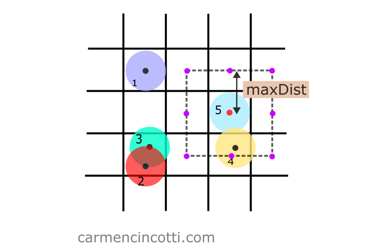
As you can see, I’ve marked all points that we’ll eventually query as violet.
Now, we’ll loop through all of these violet points in order to see if the squares in which they reside contains particles. We’ll also need to check the square that particle resides in.
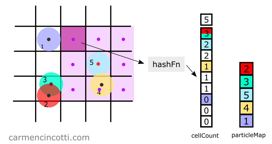
For now, let’s see an example on how to check for particles within a square of interest. I’ll query the top left violet point.
I’m going to query the purple point at the top left. We start by calculating the coordinate of the grid, squareCoordinate, in which this point is located. To do this, we use the intCoord function:
intCoord(pos: number) {
    return Math.floor(pos / spacing);
}

const squareCoordinates = [
    intCoord(pos.x),
    intCoord(pos.y),
]
Using squareCoordinate, we can index into cellCount to see what particles are there…
Recall that we can use the hash function hashPos to compute the hash of a position:
hashCoords(xi: number, yi: number, zi: number) {
    const hash = (xi * 92837111) ^ (yi * 689287499) ^ (zi * 283923481);
    return Math.abs(hash);
}

hashPos(squareCoordinates) {
    return hashCoords(
        ...squareCoordinates
    );
}
Assume that we use a hash function that, by hashing squareCoordinate, the index is returned to us :
To see if there are particles in this space, we carry out the following calculation:
where is the index that we just calculated.
Continuing this example, we find that there is nothing in the table at index !:
Now, let’s see an example of a square in which particles reside. Let’s query the coordinate located at the bottom:
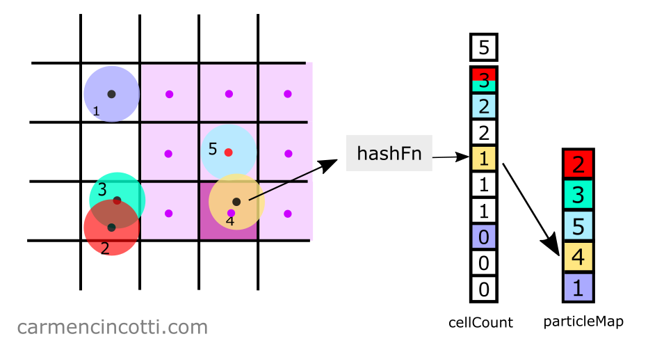
By hashing squareCoordinate, we get the index . With this index, we query the cellCount array for particles as before:
This time, we see that one particle does exist within the square of interest! The number at cellCount[i] also acts as the index into particleMap, which in this case is .
Therefore, by indexing into particleMap with the index , we are able to see that particle is within the square of interest.
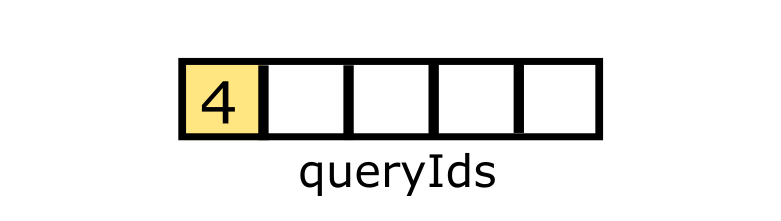
To finish up, we add the particle in an array called queryIds to use it later in the application:
Step 3: Confirmation of the collision
With our array, queryIds, it’s time to confirm that each particle found in the previous step falls within the maximum search distance, maxDist, from the particle of interest, in this case particle :
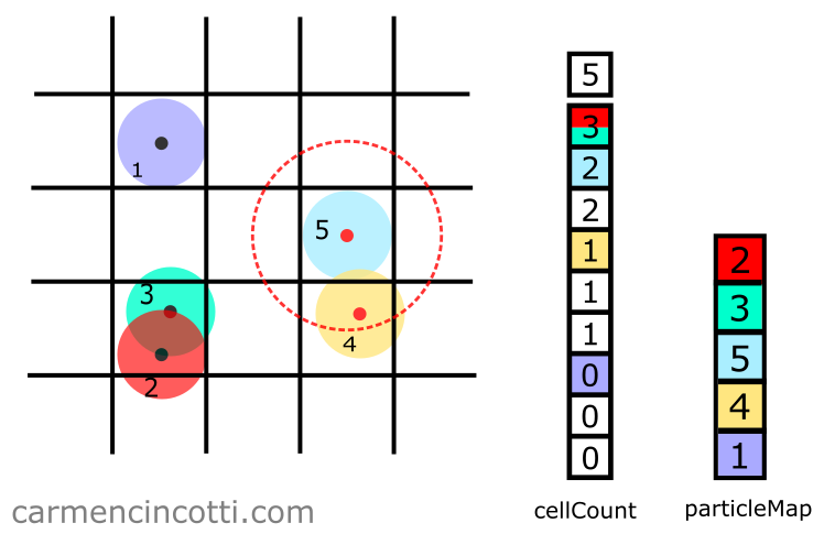
We see in the image above that the particle is indeed within this search radius. In the code, we need to use a distance function to confirm this is the case. We can use a typical distance function, like so:
If , we can consider that the two particles intersect!
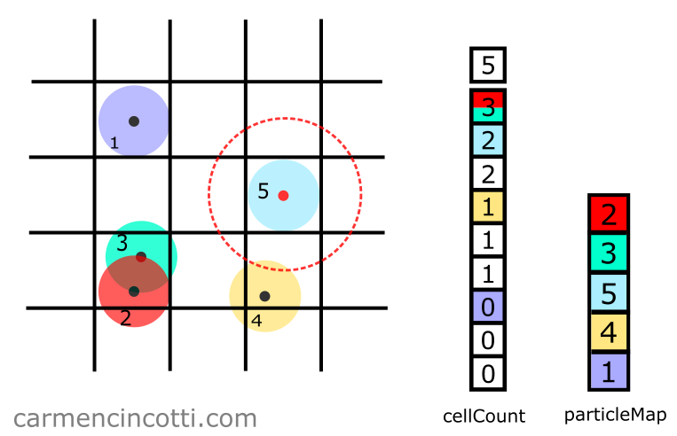
If , we would notice that the two particles do not intersect, just like as represented in the image below:
Of course, we can avoid these steps by using two loops to visit all the particles twice in order to determine if two particles intersect. Such an operation would have a time complexity . However, during a simulation, such complexity is not acceptable.