The Isometric Bending Constraint | XPBD

XPBD uses particle constraints to ensure that particles move in a certain manner, relative to other particles. Let's take a deeper look into a common constrant that we'll find in a cloth simulation, the isometric bending constraint.

Keywords: position based dynamics, cloth simulation, lagrange, physics, computer graphics

By Carmen Cincotti

August 29, 2022Updated September 12, 2022

A summary of XPBD
Satisfying the constraints
Isometric bending constraint
- How to find the cotangent between two vectors 🤔
The code
Resources

A big piece of the XPBD puzzle, which we already talked about a few weeks ago, is the satisfaction of particle constraints. Particle constraints force a particle to move in a certain way, relative to the other particles in the system.

How a particle moves back to the string

If you’ve been following me for the past few months, you most likely know of my goal to simulate fabric 🧵. Last week, we talked about distance constraints. This week, we’ll be focusing on isometric bending constraints.

Here are once again those famous articles that we already studied together during an article from a few weeks ago on XPBD that I will reference for the math during this post:

A summary of XPBD

Recall that the XPBD algorithm with small steps is defined as follows:

Algorithm of XPBD with small steps

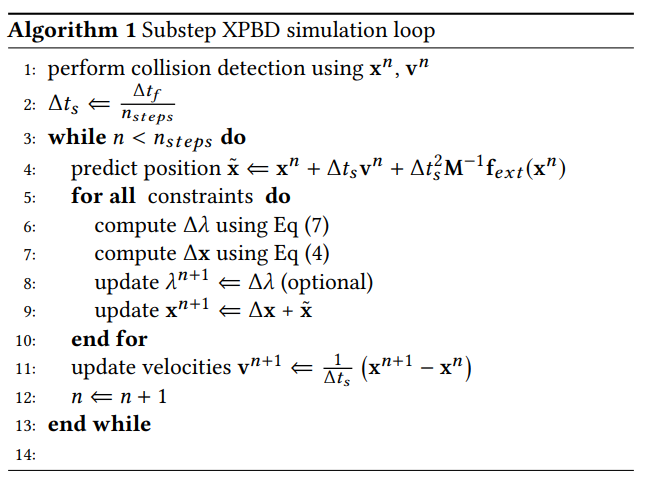
⚠️ As I said, we have already covered this algorithm thoroughly, and I recommend that you read the article if you are already lost.

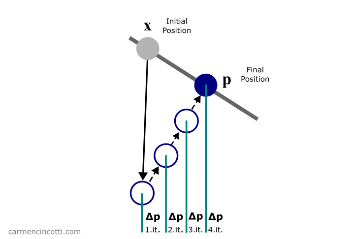
For now, we are only interested in the loop that is in lines (6) - (11). As you can see, the function of this loop is to satisfy the constraints of the simulation in order to directly correct the positions of each particle that participates in the constraints.

We just covered the reason why this simulation method is called as Position Based Dynamics - PBD 🎉.

Satisfying the constraints

Our objective during the loop is to calculate the correction vector that a particle must move in order to satisfy, or come closer to satisfying, the constraints.

\Delta \mathbf{x} = \Delta \lambda \mathbf{M}^{-1} \nabla C \mathbf{x}^T

where $\Delta \lambda$ is defined as:

\Delta \lambda = \frac{-C(\mathbf{x})}{\nabla C(\mathbf{x}) \mathbf{M}^{-1} \nabla C(\mathbf{x})^T + \tilde{\alpha}}

Note that $\tilde{\alpha} = \frac{\alpha}{\Delta t^2}$ where $\alpha$ is the constraint compliance. Recall that $\alpha = \frac{1}{k}$ where $k$ is the stiffness of the constraint. $C(\mathbf{x})$ is the constraint equation, $\nabla C(\mathbf{x})$ is the gradient of $\nabla C(\mathbf{x})$ and is therefore a vector. $\mathbf{M}^{-1}$ is a diagonal matrix of inverse masses of the particles participating in the constraint.

$\Delta \lambda$ , $C(\mathbf{x})$ , and $\tilde{\alpha}$ are scalar values.

Using these equations, we will simulate some constraints with code! 💻

Isometric bending constraint

Let’s now talk about the isometric bending constraint. Here is an example of what that might look like during a cloth simulation:

Bending cloth example

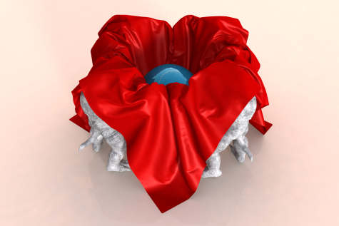
The isometric bending constraint is a bending constraint for inextensible surfaces. Basically, it’s a great bending model for cloth simulations due to the fact that cloth cannot normally be stretched (although that depends on the material).

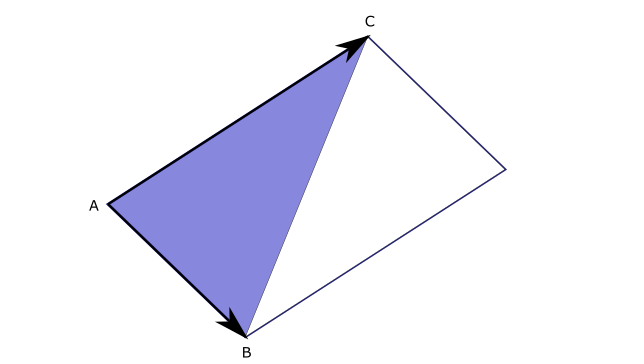
The constraint consists of four particles that form a configuration of two triangles, which looks like the following:

Four triangles configuration

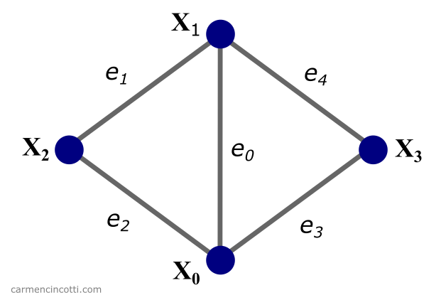
where each purple circle is a particle at a location $\mathbf{x}_n$ . Edges of the two triangles are labeled as $e_n$ . This configuration is called a stencil.

To calculate the necessary displacement of a particle in order to satisfy the constraint - we first start with the isometric bending constraint equation:

C_{bend}(\mathbf{x}_s) = \frac{1}{2}\sum_{i,j}\mathbf{Q}_{i,j}\mathbf{x}_{i}^T\mathbf{x}_{j}

What 😨?! Don’t worry, we’ll break this equation down little by little.

We start with the matrix $\mathbf{Q}_{i,j} \in \mathbb{R}^{\text{4x4}}$ , which is the local constant Hessian bending energy. This resource gives the derivation.

We initialize the matrix $\mathbf{Q}$ only once for each configuration of four particles. Recall that the Hessian matrix includes the second order partial derivatives:

\mathbf{Q}_{i,j}(f) = \frac{\partial^2 f}{\partial{x}_i\partial{x}_j}

where $A_0$ and $A_1$ are areas of adjacent triangles. Recall that we can find the area of a triangle if the locations of it’s three points are given with a small linear algebra trick:

Finding area of triangle with cross product

A = \frac{1}{2}|\vec{AB} \times \vec{AC}|

$\mathbf{K}$ is a vector which consists of the cotangents between the triangle edges $c_{jk} = \cot\angle e_j,e_k$ :

\mathbf{K} = [c_{01} + c_{04}, c_{02} + c_{03}, -c_{01} - c_{02}, -c_{03} - c_{04}]

How to find the cotangent between two vectors 🤔

The cotangent is defined as follows:

\cot \theta = \frac{\cos \theta}{\sin \theta}

We can find $\cos \theta$ with the dot product:

\mathbf{a} \cdot \mathbf{b} = |\mathbf{a}| \times |\mathbf{b}| \times \cos \theta \\[6pt] \therefore \cos \theta = \frac{\mathbf{a} \cdot \mathbf{b}}{|\mathbf{a}| \times |\mathbf{b}|}

To find $\sin \theta$ , we use the cross product:

|\mathbf{a} \times \mathbf{b}| = |\mathbf{a}| |\mathbf{b}| \sin \theta \\[6pt] \therefore \sin \theta = \frac{|\mathbf{a} \times \mathbf{b}|}{|\mathbf{a}| \times |\mathbf{b}|}

We can therefore rewrite the equation for $\cot \theta$ as follows:

\cot \theta = \frac{\cos \theta}{\sin \theta} \\[6pt] = \frac{\frac{\mathbf{a} \cdot \mathbf{b}}{|\mathbf{a}| \times |\mathbf{b}|}}{\frac{|\mathbf{a} \times \mathbf{b}|}{|\mathbf{a}| \times |\mathbf{b}|}} \\[6pt] = \frac{\mathbf{a} \cdot \mathbf{b}}{|\mathbf{a} \times \mathbf{b}|}

Let us now go back to this equation:

C_{bend}(\mathbf{x}_s) = \frac{1}{2}\sum_{i,j}\mathbf{Q}_{i,j}\mathbf{x}_{i}^T\mathbf{x}_{j}

$\mathbf{x}$ is the location of the particles. Finally, we need the gradient $\nabla C_{bend}$ to find $\Delta \lambda$ which is defined as follows:

\nabla C_{bend} = \sum_{j}\mathbf{Q}_{i,j}\mathbf{x}_{j}

We now have all the equations that we need. I find that these equations are difficult to truly grasp without seeing them at work in the code. So, let’s look at some code now!

The code

If you have already seen the code for the distance constraint from the last article, you will notice that the simulation loop does not change. We are just concerned with the bendingConstraint function.

Fortunately, the code is not rocket science. First we need to calculate C, then the gradient - grad, which is $\nabla C$ . Then we find deltaLagrangianMultiplier which is $\Delta \lambda$ . Finally, we find $\Delta \mathbf{x}$ , which is the displacement of a particle during a substep in time.

When running the program - we should see the following logged to the console:

BEFORE APPLYING XPBD LOOP
-------------------------


POSITION P1:  [ '0.0000', '0.0000', '0.0000' ] 
POSITION P2:  [ '0.0000', '1.0000', '0.0000' ] 
POSITION P3:  [ '-0.5000', '0.5000', '0.0000' ] 
POSITION P4:  [ '0.5000', '0.5000', '0.0000' ]


VELOCITY P1:  [ '0.0000', '0.0000', '0.0000' ] 
VELOCITY P2:  [ '0.0000', '0.0000', '0.0000' ] 
VELOCITY P3:  [ '0.0000', '0.0000', '0.0000' ] 
VELOCITY P4:  [ '0.0000', '0.0000', '0.0000' ]

AFTER APPLYING XPBD LOOP
------------------------


POSITION P1:  [ '0.0000', '0.0000', '0.0000' ] 
POSITION P2:  [ '0.0000', '1.0000', '0.0000' ] 
POSITION P3:  [ '-0.5000', '0.5000', '0.0000' ] 
POSITION P4:  [ '0.5000', '0.5000', '0.0000' ]


VELOCITY P1:  [ '0.0000', '0.0000', '0.0000' ] 
VELOCITY P2:  [ '0.0000', '0.0000', '0.0000' ] 
VELOCITY P3:  [ '0.0000', '0.0000', '0.0000' ] 
VELOCITY P4:  [ '0.0000', '0.0000', '0.0000' ]

Great! All that remains is to integrate these constraints into the fabric simulation! See you then!

Carmen's Graphics Blog

The Isometric Bending Constraint | XPBD

A summary of XPBD

Satisfying the constraints

Isometric bending constraint

How to find the cotangent between two vectors 🤔

The code

Resources

Comments for The Isometric Bending Constraint | XPBD

Contribute